• Latest Version, 2024 Assessment
• 2018 assessment

Intertidal Community Temperature Index

Over two decades since 2002 there have been relatively small changes in the intertidal benthic community index, in line with expectations from the changes in sea surface temperature in the region. However, rapid increases in sea surface temperature, with 2022 and 2023 being the warmest on record, suggests that the change in community composition in the coming decade will be much larger. 

Background

The UK Intertidal Community Temperature Index (CTI) is a measure of the status of a community in terms of its composition of cold and warm water species. It is quantitative, easily applied, and gives a direct measurement of the response to climate change driven by increased sea surface temperature across all the species in a community. The index builds on a solid foundation of understanding of changes in species abundance and presence in relation to patterns of temperature across geographical scales and over time. This information is essential to understand how anthropogenic pressure exacerbates effects from climate change. 

The UK CTI is an indicator developed from the Marine Biodiversity and Climate Change (MarClim) time-series. The MarClim project carries out annual surveys of 100 rocky intertidal shores around the UK. The dataset comprises species of macroalgae and invertebrates that are foundation species, ecosystem engineers, and keystone species for intertidal habitats. Community Temperature Index values have been calculated for 3,117 rocky shore surveys around the UK since 2002. 

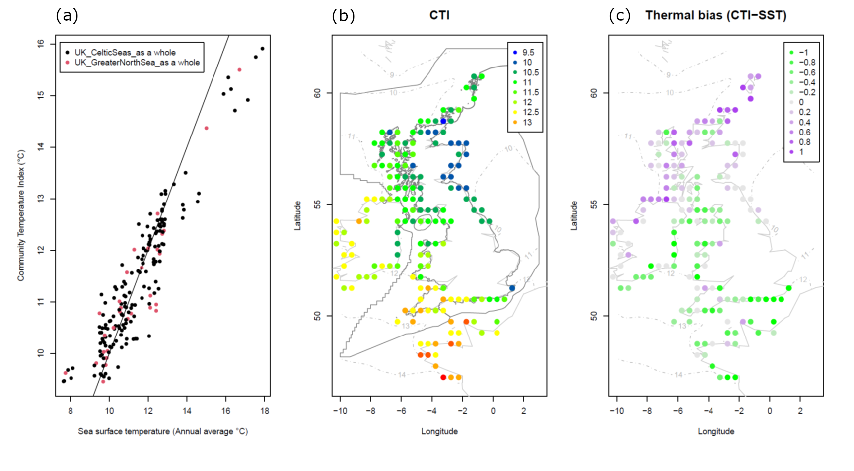
Figure 1. Community Temperature Index (CTI) patterns in MarClim data from 2002 to 2022. (a) CTI versus average annual sea surface temperature (NOAA OISSTHR V2 1982-2018) averaged in 0.5° latitude/longitude grid cells. (b) CTI values averaged in 0.5° latitude/longitude grid cells.  (c) The difference between average CTI and local average sea surface temperature, termed ‘Thermal Bias’, in 0.5° latitude/longitude grid cells. 

Since 2010, MarClim surveys have taken place annually in England and Wales. In Scotland, surveys were completed in 2014-2015 and 2020-2022. Surveys in Northern Ireland were done in the early phase of the programme from 2002-2006. 

The coverage of the MarClim programme surveys has allowed comparison of the changes in composition of rocky shore communities over decadal time periods, between 2002-2010 and 2011-2022. 

Figure 2. Daily sea surface temperature anomalies for 55°N-61N, 6W-0W from NOAA OISSTHR V2 from 1982 to 2022, showing decadal and annual trends in temperature. Anomalies are expressed relative average temperatures for each day of the year for a 1983-2012 baseline. Comparison periods for MarClim data are shown as shaded polygons. 

Intertidal surveys using the MarClim protocols have spanned the Atlantic coast of Europe from Portugal to Norway since 2002 (Figure 1). In the northern North Sea, temperatures have remained relatively stable since the start of the programme (Figure 2). 

 

Further information

UK Target on Intertidal Community Temperature Index 

This indicator is used to assess progress against the following target, which is set in the UK Marine Strategy Part 1: The extent of adverse effects caused by human activities on the condition, function and ecosystem processes of habitats is minimised. However, a full assessment against this target is not possible at this stage. 

Key pressures and impacts 

Climate change is one the key pressures driving biodiversity loss and ecosystem service changes. The impacts on marine organisms can be either direct by impacting their physiology or indirect through changes in distribution of prey/predators. Intertidal and shallow habitats in particular are likely to be significantly impacted through sea level rise and temperature change. 

Measures taken to address the impacts 

Measures to protect intertidal benthic habitats are set out in the latest UK Marine Strategy Part 3. These include the Habitat Regulations, Water Environment Regulations (WER) River Basin Management Plans, Urban Wastewater Treatment Directive, Nitrates Directive, The Convention for the Protection of the Marine Environment of the North-East Atlantic (OSPAR) measures on species and habitats, Marine Spatial Planning, land management schemes, catchment sensitive farming and European Marine Site management schemes. 

Monitoring, assessment and regional co-operation 

Areas that have been assessed 

This indicator is only applicable to rocky intertidal areas. 

Assessment thresholds 

The Community Temperature Index has not been assessed against a threshold related to Good Environmental Status. 

Regional co-operation  

The indicator has not been used for the OSPAR Quality Status Report (2023), but it may be used for future regional analyses as part of the work under the Intersessional Correspondence Group on the Coordination of Biodiversity Assessment and Monitoring (ICG-COBAM) and the Working Group on Changing Ocean Climate and Ocean Acidification (WG COCOA).  

Assessment method

Indicator metric 

The Community Temperature Index (CTI) is a measure of the status of a community in terms of its species composition of cold- and warm-water species (Devictor and others, 2008) and gives a direct measurement of the response to climate and climate change across all species in a community. The index builds on a solid foundation of understanding of changes in species abundance and presence in relation to patterns of temperature spatially and temporally. The CTI uses the MarClim time-series; a dataset comprised of species records of macroalgae and invertebrates from rocky intertidal habitats. 

The first step in producing the CTI is the collation of information on the distribution of each species in the community to obtain the Species Temperature Index. Species distributions for the most frequently recorded UK rocky intertidal species have been compiled from literature and online sources. The Species Temperature Index is defined as the midpoint temperature value of the global geographical range for each of the species. This is the thermal midpoint of the species range: the median or 50th percentile of within-range temperatures. Species Temperature Index is usually calculated by identifying reliable sources of information on distributions of the component species, for example, the distribution of Poli's stellate barnacle (Chthamalus stellatus) in relation to average sea surface temperature is shown in Figure 3. Without a comprehensive pre-existing set of global distribution maps, the approach adopted for UK intertidal species was to examine the literature on the biogeography of each species one by one and create Geographic Information System polygon shapefiles that encompass areas where the species is known to occur. The Species Temperature Index effectively separates cold-water from warm-water species, and values range from 5.0⁰C for the Boreal Arctic barnacle (Balanus crenatus), a cold-water species, to 19.0⁰C for the purple sea urchin (Paracentrotus lividus), a warm-water species. 

Figure 3. The global distribution of Poli's stellate barnacle (Chthamalus stellatus) shown as an orange polygon overlay on sea surface temperature contours of annual averages between 1982 and 2011 from NOAA OISST V2. 

CTI values for the community data collected under the MarClim programme were calculated using methods outlined in (Burrows and others, 2020). The CTI is expressed in degrees Celsius and is calculated from the average species temperature index of all species in a community, weighted by their abundance. The CTI is a single value for a community of n species, calculated as the average of all the species’ Species Temperature Index values (STI or T_i), weighted by their abundance (w_i) and expressed in degrees Celsius. Thus: 

For MarClim data, abundance was expressed as the rank of the abundance category on the SACFOR scale, with Absence as 0, Rare as 1, Occasional as 2, Frequent as 3, Common as 4, Abundant as 5 and Super Abundant as 6. CTI values were calculated for every individual survey except for those with fewer than 10 species. Declines in abundance of cold-water species (lower T_i values) and increases in abundance of warm-water ones (higher T_i) result in an increase in Community Temperature Index, an expected response to climatic warming. 

Two methods were used to aggregate and compare survey results across the UK and from the UK Marine Strategy sub-regions, the Celtic Seas and the Greater North Sea. The methods were designed to reduce the influence of differences in survey coverage between comparison periods and to allow investigation of the contribution of individual species to any observed changes in composition. 

Community changes 

In the first approach, CTI values were calculated for each survey using the abundance of all species with known Species Temperature Index values (Method 1). Survey CTIs were combined into CTI maps by averaging site-level CTIs over 0.5° latitude/longitude grids for each time period (2002-2010 versus 2011-2022). Maps were then created of the difference in CTI between the two time periods to show the change in each 0.5° latitude/longitude grid cell. Changes in CTI between periods were analysed using map data as 0.5° grid values with absolute changes assessed using confidence intervals of mean values for comparisons among regions.  

Species changes 

To investigate the influence of species-level changes in abundance on CTI change, spatially matched groups of surveys were compared across time periods (Method 2). Abundance values for each species were averaged across the same 0.5° latitude/longitude grid cells in each time period. Only abundance values from grid cells surveyed in both periods were used in comparisons. Averages of the difference in abundance were calculated for the two UK Marine Strategy sub-regions by combining data from the two main teams of surveyors (Marine Biological Association (MBA) and Scottish Association of Marine Science (SAMS)). Relationships between species changes and the range of global temperatures that each species occupies (their thermal affinities) in each region were assessed for evidence of changes in abundance being driven by a response to changes in temperature. CTI values for each 0.5° latitude/longitude grid cell were calculated from these aggregated species abundance values to check for correspondence with CTIs derived from survey-level CTIs. Small differences between the two methods (average of survey-level CTIs; CTI from average species abundance) were expected because of the different ways that data were aggregated. 

Data used and quality assurance 

Survey sites used in the MarClim project are located in areas of extensive, exposed intertidal rocky reef or artificial hard coastal structures or defences, away from areas of coastline heavily developed or utilised for social or economic purposes, and avoiding riverine and estuarine outputs. Rocky shore species (49 species of ectothermic (cold-blooded) invertebrates and 35 species of macroalgae) assessed during MarClim surveys are recorded using the SACFOR scale 

Knowledge of the distribution of CTI anomalies over time from long-term monitoring sites allows determination of the minimum number of survey sites required to detect a given change in the CTI value. This represents a given shift in community thermal trait composition with a specified level of detectability and statistical significance (in this case p=0.05). Detectability is otherwise known as the power of the test (1 - β, where β is Type II error: the probability of erroneously accepting an otherwise false null hypothesis of no change). This minimum number of sites for a given change in temperature and level of significance critically depends on the standard deviation of the anomalies. For example, for the sites in the south-west of England from 2002 to 2014, the standard deviation of anomalies was 0.409⁰C, giving a range of numbers of paired surveys needed to detect a change in the CTI of a given magnitude: 22 sites are required to detect a change of 0.3⁰C with a power of 0.9). Many more than 22 sites were surveyed in both time periods. 

Uncertainty in CTI estimates is generated by the randomness of species encountered at each survey site. This can be distinguished from uncertainty produced by the surveys themselves. For MarClim surveys, additional uncertainty is generated by the variable application of survey methods, differences in effort across shore levels and among taxa, mistakes in identification and varying levels of taxonomic skill across surveyors (Burrows and others, 2014). Where cross-calibration among surveyors has been done (Burrows and others, 2017), levels of similarity for abundance estimates and species richness are reassuringly high: 83% of SACFOR abundance estimates are within one category and 92% within two categories. 

For single surveys, a useful estimate of uncertainty is derived from the standard deviation of the STI values divided by the square root of the number of species in the community: the standard error of CTI. 95% confidence intervals for CTI can be calculated by multiplying the standard error by the appropriate Student’s t value (for p=0.05 and n-1 where n is the number of species in the community). A full description of the method can be found in Burrows and others (2020). 

Results

Changes in CTI values from 2002 to 2022 are shown in Figure 4, and listed for each UK Marine Strategy sub-region in Table 1.

Figure 4. CTI difference map comparing surveys in 2002-2010 with those from 2011-2022. The map shows change in CTI values between the two periods in 0.5° latitude/longitude grid cells. CTI declined overall (mean change -0.25°C, 95% CL -0.17 to -0.34, P=0.01). Only data from surveys with >10 species recorded were used. Black circles show MarClim survey locations over the entire period (2002-2022). 

Table 1. Statistical tests of change in CTI values between 2002-2010 and 2011-2022 across both UK Marine Strategy sub-regions. Changes in CTI were assessed using values of CTI individual surveys aggregated in 0.5° latitude/longitude cells and paired across the two periods. Changes are shown as averages and 95% confidence intervals (from standard errors and t-values associated with the number of comparisons per region, number of 0.5° latitude/longitude cells (Ncells)).  

	Celtic Seas			Greater North Sea			All UK
Difference in	Mean	Lower 95% CL	Upper 95% CL	Mean	Lower 95% CL	Upper 95% CL	Mean	Lower 95% CL	Upper 95% CL
All Species	-0.292	-0.391	-0.193	-0.156	-0.326	0.014	-0.251	-0.336	-0.166
CTI
Benthic	-0.162	-0.346	0.022	-0.046	-0.381	0.289	-0.127	-0.287	0.033
invertebrates
aCTI
Macroalgae mCTI	0.011	-0.076	0.098	-0.021	-0.101	0.059	0.001	-0.063	0.066
Ncells	58			29			87

Changes in Community Temperature Index (CTI) from 2002-2010 to 2011-2022 

• Changes in CTI of rocky shore communities around the coastline of the UK over the two decades have been relatively small and in line with expectations from the changes in sea surface temperature in the region. 

• For 2011-2022 compared with 2002-2010, although there were geographical variations, CTI declined across the whole of the UK (0.25°C) with a shift in community composition towards cold-water species. This in line with the small negative trend in sea surface temperature seen in the southwest (Burrows et al., 2020) and northern UK (Figure 2) over the two decades, particularly between 2002 when the surveys began and the early 2010s with the cold winters of 2009/10 and 2011/12. 

• The change in CTI based on invertebrate species showed a small decline in CTI across the UK (0.13°C), but not significantly different from no change. 

• For macroalgae, there was no overall change in CTI across the UK 

Further information

Changes in Community Temperature Index from 2002-2010 to 2011-2022 

Between 2002-2010 and 2011-2022, based on average CTI from surveys (Figure 4), CTI showed a decline across the UK (Table 1, 0.25°C) with a shift in community composition towards cold-water species. The change in CTI based on benthic invertebrate species (aCTI) showed a small decline in CTI across the UK (0.13°C, Table 1), but this was not significantly different from no change. There were some geographically variable responses in the north. Northeast Scotland (Figure 5a) saw increased CTI for benthic invertebrate species, but western coasts of Scotland had declines in CTI based on benthic invertebrate species between the two periods. For macroalgae, there was no overall change in CTI across the UK (Figure 5b). 

Figure 5. CTI difference maps for (a) benthic invertebrates and (b) macroalgae based on comparing surveys in 2002-2010 with those from 2011-2022.   

CTI changes between 2002-2010 and 2011-2022 were similar across the UK Marine Strategy sub-regions: rocky shore communities in the Celtic Seas region showed a cooling response (Table 1, Figure 4: -0.29°C) and those in the Greater North Sea showed a similar shift towards dominance by cold water species (Table 1, Figure 4: 0.16°C, albeit varying according to the methods of calculation. The mean CTI was lower in the Celtic Seas compared to the Greater North Sea, but the results did not show a strong statistical difference.  Changes in CTI based on macroalgae were negligible in both regions. 

Species-level changes: 2002-2010 to 2011-2022 

Although overall changes in CTI based on macroalgae were negligible, some species showed changes in abundance. Fucus vesiculosus increased by more than one SACFOR category in both regions between the decades (Figure 6a), with increases in Fucus spiralis and Fucus serratus also evident. When expressed as the change in proportional contribution to total abundance of community species (Figure 6b), the changes in some species were less evident (Figure 6b). Changes in absolute abundance were strongly related to their change proportional contribution (Figure 6b).   

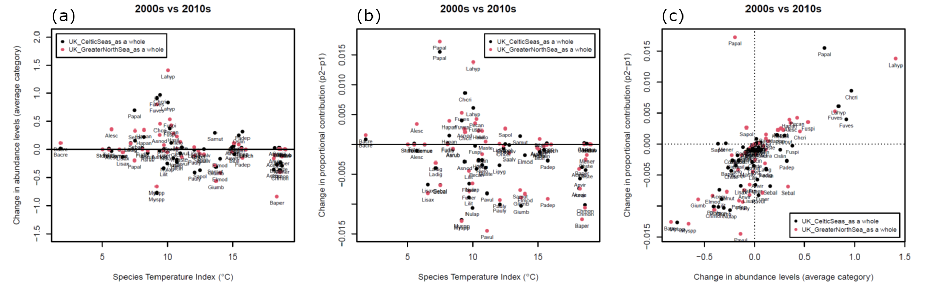
Figure 6. Changes in species abundance from surveys in 2002-2010 to 2011-2022. Data were divided into UK Marine Strategy sub-regions (Celtic Seas and Greater North Sea). Abundance values for each species were averaged into 0.5° latitude/longitude grid cells in each period. Only abundance values from grid cells surveyed at least twice in both periods were used in comparisons. Plots show (a) change in average abundance between periods for each region plotted against Species Temperature Index, (b) change in proportional contribution to the community between periods against Species Temperature Index, and (c) changes in average abundance and proportional contributions together. Abbreviations Acequ, Actinia equina; Acfra, Actinia fragacea; Alesc, Alaria esculenta; Anvir, Anemonia viridis; Asnod, Ascophyllum nodosum; Asrub, Asterias rubens; Auver, Aulactinia verrucosa; Bacre, Balanus crenatus; Baper, Balanus perforatus; Bibif, Bifurcaria bifurcata; Caziz, Calliostoma zizphinum; Chcri, Chondrus crispus; Chmon, Chthamalus montagui; Chste, Chthamalus stellatus; Clery, Clibanarius erythropus; Cospp, Codium sp; Elmod, Austrominius modestus; Fudis, Fucus distichus; Fuser, Fucus serratus; Fuspi, Fucus spiralis; Fuves, Fucus vesiculosus; Gicin, Steromphala cineraria; Gipen, Steromphala pennanti; Giumb, Steromphala umbilicalis; Hapan, Halichondria panicea; Hasil, Halidrys siliquosa; Hatub, Haliotis tuberculata; Hielo, Himanthalia elongata; Ladig, Laminaria digitata; Lahyp, Laminaria hyperborea; Laoch, Laminaria ochroleuca; Lemue, Leptasterias muelleri; Lilit, Littorina littorea; Lipyg, Lichina pygmaea; Lisax, Littorina saxatilis; Maste, Mastocarpus stellatus; Mener, Melarhaphe neritoides; Myspp, Mytilus edulis; Nulap, Nucella lapillus; Oncel, Onchidella celtica; Oslin, Phorcus lineatus; Padep, Patella depressa; Paliv, Paracentrotus lividus; Papal, Palmaria palmata; Pauly, Patella ulyssiponensis; Pavul, Patella vulgata; Pecan, Pelvetia canaliculata; Saalv, Sabellaria alveolata; Samut, Sargassum muticum; Sapol, Saccorhiza polyschides; Sebal, Semibalanus balanoides; Stdro, Strongylocentrotus droebachiensis; Tetes, Testudinalia testudinalis. 

Conclusions

Changes in CTI of rocky shore communities around the coastline of the UK over the two decades have been relatively small and in line with expectations from the changes in sea surface temperature in the region. Rapid increases in sea surface temperature over the first two years of the 2020s, with 2022 and 2023 being the warmest on record, suggest that the change in community composition in the coming decade will be much larger. The first 20 years of this programme will serve as a solid baseline for detection of change. 

Further information

The magnitude of change in CTI relative to temperature change 

Change in CTI between 2002-2010 and 2011-2022 seen in the dataset (-0.25°C) was in line with the small negative trend in sea surface temperature seen in the southwest (Burrows and others, 2020) and northern UK (Figure 2) over the two decades, particularly between 2002 when the surveys began and the early 2010s with the cold winters of 2009/10 and 2011/12. Temperatures rose slightly after this point to levels seen though the mid-2000s and only exceeded those in the early 2000s after 2020. The decline in CTI over the period in this analysis was also evident in the analysis by Burrows and others (2020) using annual time series from repeatedly surveyed sites in the southwest. Given the lack of a strong trend in temperature over the period of the surveys, it is therefore not surprising that the changes in community composition over time shown using the CTI approach have been small and hard to detect. The CTI method does, however, successfully describe the changes across the latitudinal gradient in sea temperature (Figure 1b). This may be because the magnitude of differences in temperature along latitudinal gradients is greater than that yet seen over time in the same location between the two decades of the MarClim programme.  

Regional variations in compositional change 

Regional and smaller-scale variations in CTI change may reflect regional differences in warming over the two comparison periods. However, it must be remembered that for the first decade, sampling was not synchronised across regions. Surveys in the northern UK were organised into annual field campaigns to specific areas in the 2000s, so the apparent local-scale patterns in CTI change between 2002-2010 and 2011-2022 may be a result of sampling areas in different years of the decade.  

As a future strategy for detecting compositional change across the rocky shores of the UK using MarClim protocols, the ideal approach would be to revisit exactly the same sites and the same species list for comparing CTIs and species abundance changes between periods for comparison. The method used here attempts to reduce the effects of variable sampling locations and species lists on change between periods and may be a reasonable compromise in the absence of ideal datasets. It is recommended that in the absence of spatially matched surveys and consistent species recording, CTI changes based on survey-level CTIs aggregated across larger areas (0.5° latitude/longitude grid cells) should be used for detecting changes in CTI, with CTI based on regional average changes in species abundance to show how groups of species respond to climate change. 

The approach is versatile, being able to accommodate different kinds of data from presence-only records to detailed abundance estimates and is well suited to the categorical abundance methods used on rocky shore for many decades. 

Knowledge gaps

The key knowledge gaps are: 

• Data are only available for a limited number of species during different time periods. 

• Lower frequency of surveys in some areas (Scotland and Northern Ireland) reduces confidence in detection of longer-term trends. 

• Sampling not always synchronised across regions. 

• The CTI has not been assessed against a threshold related to Good Environmental Status. 

Further information

Data limitations 

A difficult problem is when data are only available for a limited number of species during different time periods. In early surveys around the UK, the focus was often on species distributions, for example, Southward and Crisp (1954) often sampled only the climate-sensitive species, such as the topshells of the genus Osilinus and Steromphala, the barnacles Semibalanus and Chthamalus and the patelid limpets. Variable numbers of species will have a strong influence on CTI estimates and further methods of dealing with this issue are needed before the application to earlier datasets from the 1950s onwards. Another drawback is that the specific mechanisms driving changes are not immediately obvious, mostly since the approach ‘averages out’ responses across such a wide range of species. This area is beginning to yield some more insight, for example, responses to climate by species are emerging as critically dependent on the location within the species range, with species in the cold half of their range responding positively to warming, while those in their warm half responding negatively. 

Ideally, the approach would be to revisit exactly the same sites and the same species list for comparing CTIs and species abundance changes between periods for comparison. However, in the absence of ideal datasets, the method used here of aggregating survey-level CTIs across larger areas, attempts to reduce the effects of variable sampling locations and species lists on change between periods. 

Analysis issues 

Unlike analysis of time series of repeated surveys at single locations, comparing map-based data on community composition over time requires careful consideration of how to best match the sets of data. Varying survey locations among comparison periods and shifting sets of species being recorded over time and across locations both introduce errors into estimates of CTI change, as became evident in this analysis. 

Calculating CTI values for each survey and averaging those values across spatial grids (Method 1) does permit contrasts between datasets with differing sets of species. While this may be less of an issue when establishing broadscale variation in community structure (Figure 1), minor variations in species recorded can introduce error in CTI estimates at the scale of grid cells. While much of this local-scale variation may be down to variation in data collected at survey sites, it may also be due to variation in survey locations between periods. More complex statistical models that include location-specific environmental effects on communities, including wave exposure for example, could be used to account for the effects of shifting locations in detecting change.  

The Community Temperature Index can be compared with prevailing seawater temperature conditions to produce useful further measures, such as thermal bias, with implications for the sensitivity of such communities to further climatic warming, providing a unique way to assess indirect ecological effects which improve resilience to warming-related biodiversity change. 

Indicator threshold 

The CTI has not been assessed against a threshold related to Good Environmental Status. 

There are some potential options for developing an indicator threshold in the future. The CTI could be assessed in relation to the 1.5°C limit set by the 2016 Paris Agreement of the United Nations Framework Convention on Climate Change looking at past and future CTI changes in relation to temperature. This could be calculated by subtracting pre-industrial sea surface temperature values increased by 1.5°C from present CTI values, with a threshold of 0°C. Increases in CTI with climate change warming would be expected to increase the proportion of the coast which exceeds the threshold for changes under a pre-industrial plus 1.5°C. 

Linked to this, the thermal bias could also be used in future threshold calculations. Thermal bias is the difference between average CTI and local average sea surface temperature. Where the thermal bias is negative, the community is dominated by cold-water species and where thermal bias is positive, the community is dominated by warm-water species. Negative thermal bias may indicate that communities are vulnerable to the effects of warming; most species are in the cold half of their range and are likely to decline with further warming. 

References

Burrows, M.T., Mieszkowska, N., Hawkins, S.J. (2014). Marine Strategy Framework Directive Indicators for UK Rocky Shores, JNCC Report 522 (No. 522), JNCC Report. Joint Nature Conservation Committee, Peterborough, UK. 

Burrows, M.T., Twigg, G., Mieszkowska, N., Harvey, R. (2017).  ‘Marine Biodiversity and Climate Change (MarClim): Scotland 2014/15’ Scottish Natural Heritage Commissioned Report Number 939. 

Burrows, M.T., Hawkins, S.J., Moore, J.J., Adams, L., Sugden, H., Firth, L., Mieszkowska, N. (2020). Global-scale species distributions predict temperature-related changes in species composition of rocky shore communities in Britain. Global Change Biology 26, 2093–2105. https://doi.org/10.1111/gcb.14968 

Devictor, V., Julliard, R., Couvet, D., and Jiguet, F. (2008). Birds are tracking climate warming, but not fast enough. Proceedings of the Royal Society of London B: Biological Sciences, 275, 2743-2748. 

UK Marine Strategy Part One: UK updated assessment and Good Environmental Status (2019). 

https://assets.publishing.service.gov.uk/media/5f6c8369d3bf7f7238f23151/marine-strategy-part1-october19.pdf 

UK Marine Strategy Part Three: UK programme of measures (2015). 

https://assets.publishing.service.gov.uk/media/5a80330040f0b6230269218c/marine-strategy-part3-programme-of-measures.pdf 

Authors

Lead authors: Michael Burrows¹ and Nova Mieszkowska²  

Supporting authors: Marco Fusi³, Laura Pettit³ and Cristina Vina-Herbon³  

Contributors: 

Matt Service⁴, Tim Mackie⁵, Andrew Scarsbrook⁶, Edward Wright⁶, Graham Phillips⁷, Adam Britton³, Joe Kenworthy³, Kirsty Woodcock³, Lauren Molloy³, Liam Matear³, Marco Fusi³, Stefano Marra³, Steven Duncombe-Smith³, Phil Boulcott⁸, Scott Gray⁸, Eunice Pinn⁹, James Dargie⁹, Roddy MacMinn⁹, Peter Webster⁹, James Highfield¹⁰, Karen Robinson¹¹, Mike Camplin¹¹ 

¹ SAMS 

² MBA 

³ JNCC 

⁴ AFBI 

⁵ DAERA 

⁶ Defra 

⁷ Environment Agency 

⁸ Marine Directorate of the Scottish Government 

⁹ NatureScot 

¹⁰ Natural England 

¹¹ NRW 

Supported by: The Benthic Sub-Group of the Healthy and Biologically Diverse Seas Evidence Group 

Assessment metadata

Assessment Type	UK Marine Strategy Assessment Part 1 (2024)
	Benthic habitats
Point of contact email	marinestrategy@defra.gov.uk
Metadata date	Tuesday, July 1, 2025
Title	Intertidal Community Temperature Index
Resource abstract
Linkage
Conditions applying to access and use	© Crown copyright, licenced under the Open Government Licence (OGL)
Assessment Lineage	https://moat.cefas.co.uk/previous-assessments/2018-assessment/biodiversity-food-webs-and-marine-protected-areas/benthic-habitats/intertidal-community-index/
Dataset metadata	Please contact marinestrategy@defra.gov.uk
Dataset DOI	Please contact marinestrategy@defra.gov.uk

The Metadata are “data about the content, quality, condition, and other characteristics of data” (FGDC Content Standard for Digital Geospatial Metadata Workbook, Ver 2.0, May 1, 2000).

Metadata definitions

Assessment Lineage - description of data sets and method used to obtain the results of the assessment

Dataset – The datasets included in the assessment should be accessible, and reflect the exact copies or versions of the data used in the assessment. This means that if extracts from existing data were modified, filtered, or otherwise altered, then the modified data should be separately accessible, and described by metadata (acknowledging the originators of the raw data).

Dataset metadata – information on the data sources and characteristics of data sets used in the assessment (MEDIN and INSPIRE compliance).

Digital Object Identifier (DOI) – a persistent identifier to provide a link to a dataset (or other resource) on digital networks. Please note that persistent identifiers can be created/minted, even if a dataset is not directly available online.

Indicator assessment metadata – data and information about the content, quality, condition, and other characteristics of an indicator assessment.

MEDIN discovery metadata - a list of standardized information that accompanies a marine dataset and allows other people to find out what the dataset contains, where it was collected and how they can get hold of it.