
Pilot Assessment of Sentinels of the Seabed in the Celtic Seas and Greater North Sea
Seabed habitat status was assessed using a biological traits analysis method to determine impacts from bottom contacting fishing. Results indicate widespread trawling effects but with uncertainties linked to data limitations. This indicator is a pilot and subject to further development could inform future GES assessments.
Background
Anthropogenic pressures produce various types of impact on benthic habitats, including modifications to typical species composition and their functions. Therefore, monitoring the prevalence of species that are characteristic (or typical) of the habitat, that are also sensitive to a given pressure, can provide a useful tool for assessing habitat condition. Such species are referred to here as ‘sentinel species’.
The Sentinels of the Seabed (hereafter BH1) is a common indicator in OSPAR Region IV (Bay of Biscay and Iberian Coast) that has been used for the OSPAR Quality Status Report (QSR) 2023 (Plaza-Morlote and others, 2023) and is a candidate indicator in UK waters. The aim of BH1 is to assess the environmental status of a habitat using the proportional abundance of the sentinel species across pressure gradients. A biological trait analysis is required to evaluate the sensitivity of taxa to specific pressures.
It is expected that the proportion of sentinel species will decrease with increasing levels of pressure intensity. Changes in the proportion of sentinel species across a pressure gradient are used to calculate pressure-state curves for two main purposes: 1) identify tipping points and boundaries for habitat condition and 2) evaluate habitat condition. Full details of the indicator method used in the OSPAR QSR 2023 are available in the OSPAR BH1 CEMP Guidelines.
This pilot assessment is the first application of the BH1 method in UK waters. The current assessment focuses on trawling pressure which is recognised as a key pressure affecting the state of benthic communities and for which more data are available. The identification of boundaries for habitat condition based on changes in the biological community has the potential to validate and calibrate other indicators that assess impact from trawling and rely on a risk assessment approach, in particular BH3a ‘Extent of Physical Disturbance’.

Figure 1. Seapens, including Funiculina quadrangularis, and burrowing megafauna in undisturbed circalittoral fine mud. Photo credit: Keith Hiscock.
Further information
This indicator was developed within the OSPAR common indicator group of Benthic Habitats (BH) under the EU co-funded projects EcApRHA and NEA-PANACEA for Descriptor 6 (Sea Floor Integrity) and previously named ‘Typical species composition’.
The indicator method has been further developed for the OSPAR Quality Status Report 2023 (QSR 2023) and applied to assess benthic habitat conditions in in OSPAR Region IV (Bay of Biscay and Iberian Coast). The method described here reflects the latest methodology developed for the OSPAR QSR 2023 (BH1 CEMP Guidelines).
For each habitat type within a particular assessment unit, the indicator identifies a set of sentinel species from monitoring data. Sentinel species are defined as species that are characteristic of the benthic community of a habitat in reference conditions and that are particularly sensitive to the pressure evaluated. The sensitivity of individual species to the pressure is estimated using a biological traits analysis approach. Changes in the proportion of sentinel species within the benthic community are then measured across a pressure gradient to assess the level of habitat degradation.
Firstly, species that characterise a habitat are selected from least impacted area on the basis of their abundance and/or frequency of occurrence. This species list is then filtered using sensitivity indexes to select only species which are sensitive to the pressure or, if this is not possible, at least species which did not exhibit opportunistic responses. The sensitivity index used depends on the type of pressure investigated: the OSPAR QSR 2023 applied the BEnthic Sensitivity Index to Trawling Operations (BESITO) (González-Irusta and others, 2018) for the assessment of sensitivity to trawling pressure. The calculation of the BESITO index requires information on a selection of biological traits: Size, Longevity, Motility, Attachment, Benthic Position, Flexibility, Fragility and Feeding Habit. These traits are scored and combined to obtain a unique index of sensitivity.
Once the set of sentinel species has been defined, BH1 generates pressure-state curves (which correlate the proportion of sentinel species with the level of trawling impact) for each individual habitat. These curves are then applied to assess the impact of trawling pressure across these habitats, determining the level of habitat degradation after defining a quality boundary for each habitat.
Assessment method
The indicator was run using the portion of the OSPAR benthic assessment units falling within the boundaries of the UKMS sub-regions Celtic Seas and Greater North Sea (Figure 2).
For reporting purposes, results were then summarised at the scale of the UKMS sub-regions ‘Celtic Seas’ and ‘Greater North Sea’.
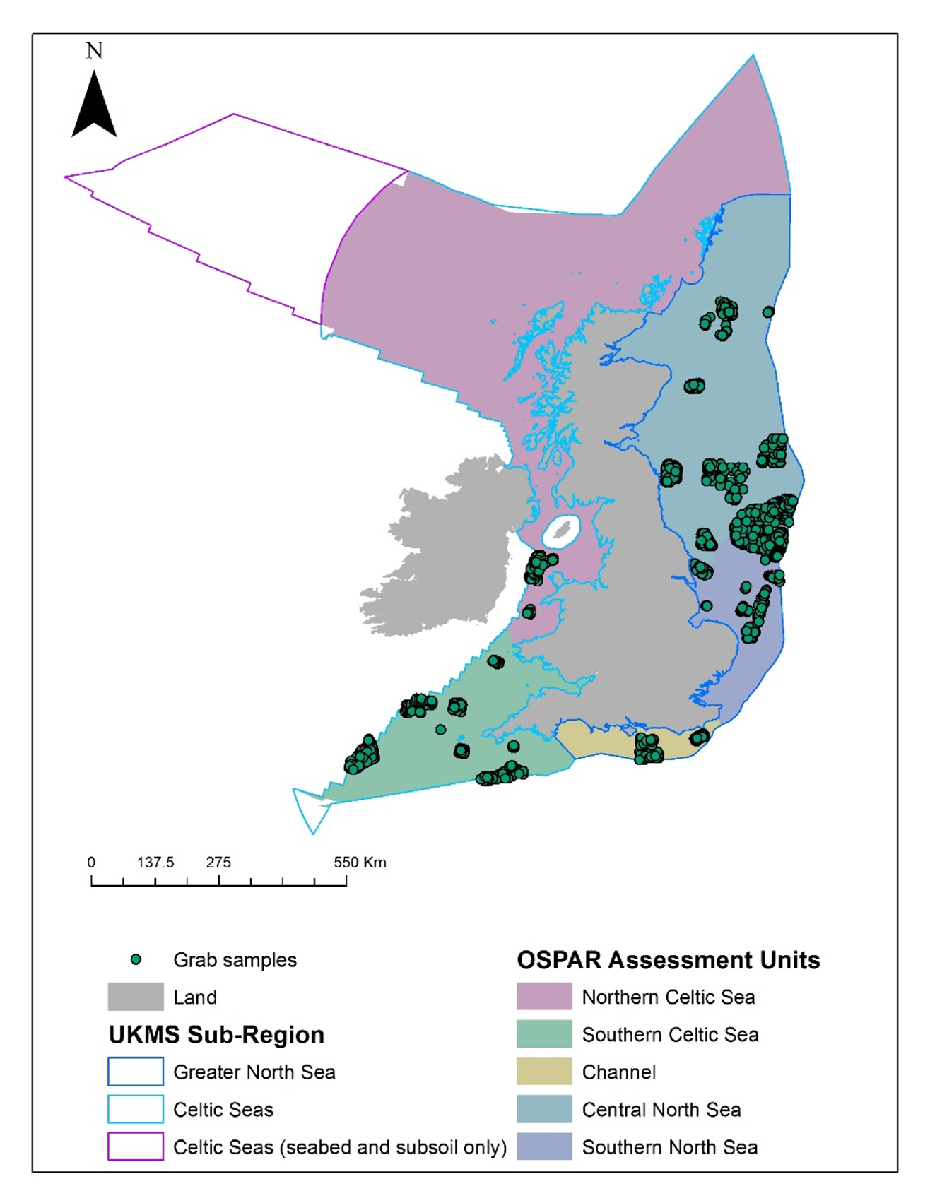
Figure 2. Distribution of biological sample data used for the BH1 Pilot assessment. Only OSPAR benthic Assessment Units containing survey data are displayed.
The indicator requires three types of information: (i) the distribution of benthic habitats, (ii) the distribution and intensity of the pressure under consideration, and (iii) biological sample data of the abundance (preferably biomass although also works with density) of benthic species from each habitat across a pressure gradient (including no pressure/low-pressure areas). These three sources of information are combined with sensitivity indexes (e.g. the BESITO index for trawling disturbance) to calculate the ecological status of a given benthic habitat.
Distribution of benthic habitats
Information on the distribution of benthic habitats was obtained from the composite habitat map (updated version of Matear and others, 2019). The composite habitat map integrates component habitat maps from both in-situ survey datasets and modelled data (in the absence of direct sample data) at the highest resolution of detail available.
Distribution and intensity of trawling pressure
The International Council for the Exploration of the Sea (ICES) abrasion layers from 2009-2020 were used to create maps showing the intensity and distribution of surface and subsurface abrasion pressure caused by towed bottom-contacting fishing gears (ICES, 2021). The data obtained from ICES contained total annual surface and subsurface Swept Area Ratio (SAR) values at a 0.05° x 0.05° ICES c-square resolution. SAR values were derived from Vessel Monitoring System (VMS) and logbook data from ICES member countries. Therefore, the dataset included VMS records for vessel greater than 15 m in length between 2009 and December 31st, 2011, and following changes to the Common Fisheries Policy (EU Council Regulation No. 44 / 2012), vessels greater than 12 m in length from January 1st, 2012, onward; vessels less than 12 m in length were not included in the dataset and VMS data were not available.
Annual SAR values within each c-square were aggregated following the method outlined in the OSPAR QSR 2023, with minor adaptations. Within this pilot assessment, both surface and subsurface abrasion pressures were analysed. Following the OSPAR QSR 2023, aggregated SAR values were calculated for each benthic sample specifically. However, within this pilot assessment aggregated SAR values were calculated as the mean SAR of four years prior to and including the sample year, rather than five (as done in the OSPAR QSR 2023). Therefore, for samples taken in 2012, the mean SAR from 2009-2012 was calculated, within the c-square the benthic sample was collected, for surface and subsurface abrasion respectively. Aggregation based on four years of pressure data, rather than five, was data driven; the earliest year of fishing pressure data available was 2009. Therefore, where benthic samples were collected in 2012, it was not possible to consider five years of pressure data, as no pressure information was available for 2008.
To facilitate identification of sentinel species later in the analysis, the BH1 assessment in OSPAR QSR 2023 categorised SAR values into five groups. However, in this pilot assessment, surface and subsurface SAR values associated with each sample were categorised into 6 groups (ranging from ‘none’ to ‘very high’) following the same approach used by the BH3a indicator ‘Extent of Physical Disturbance to Benthic Habitats‘ (Matear, and others, 2023). Categorisation of SAR values following the BH3a indicator approach enabled distinction between zero (SAR of 0, or no data reported) and very low pressure (SAR values less than or equal to 0.33), when selecting reference areas. Where sufficient benthic samples were available within a habitat in zero pressure areas, zero pressure alone could be used to represent reference conditions. However, in instances where insufficient samples were available in zero pressure areas, samples in very low pressure could also be considered, as done in the OSPAR QSR 2023 BH1 assessment (where SAR of ≤0.33 was also used to represent very low pressure). Further details on reference area identification are outlined in the ‘Selection of Sentinel Species’ section later in the method.
Biological Sample data
Data Gathering
Following the guidelines produced for the OSPAR QSR 2023, the estimation of relationships between pressure intensity and proportion of sentinel species were calculated using biomass information from monitoring data. An initial screening of potential benthic sample data was conducted by extracting from Marine Recorder (Public) snapshot (version ‘2021-08-09’) benthic sample data covering the period 2009 to 2020. This time period was selected to match available fishing pressure information.
To simplify the analyses, only infauna data collected with 0.1 m2 Hamon grabs were considered. This decision reduced any confounding factors from examining data collected with different sampling devices although it is acknowledged that this can exclude potentially usable samples collected with different sampling methods. In future iterations of this indicator, the possibility to include additional sampling devices into the analyses (such as different grab types) will be explored to increase the number of monitoring data and produce more comprehensive assessments.
As biomass was not a metric currently stored on Marine Recorder, the data extracted were then filtered to keep only sample data for which biomass information was available in the internal JNCC survey network. The resulting dataset consists of grab sample data from 29 surveys conducted at various Marine Protected Areas across five years (2012, 2013, 2014, 2016 and 2018). Survey data ingested in this assessment were largely collected offshore beyond the 12nm limit, where there is high confidence in the pressure information available. Only a negligible proportion of available samples fall along the 12 nm limit and might be affected by the reduced confidence in the pressure information (see ‘knowledge gap’ section for details). These samples were not excluded to avoid over-reducing the data available for the analyses.
Within each assessment unit, the indicator has been applied using the EUNIS 2007 classification (European Nature Information System) at Level 3 resolution.
The pilot assessment focus on the following EUNIS Level 3 habitats:
-
Sublittoral coarse sediment (A5.1)
-
Sublittoral sand (A5.2)
-
Sublittoral mud (A5.3)
-
Sublittoral mixed sediments (A5.4)
Data preparation
Some records were removed from the dataset before the analyses: juveniles, eggs, non-benthic species, records associated to inappropriate qualifier (e.g. ‘casts’, ‘fragments’) and records with very low taxonomic resolution (e.g. ‘Animalia’). The following phyla were also removed before the analyses as they include taxa not generally recorded with grab sampling, or that are not assessed for biomass consistently (Worsfold and others, 2023): Chaetognatha, Ctenophora, Entoprocta, Nematoda, Bryozoa, Phoronida, Porifera, Ciliophora, Foraminifera, Arachnida, Copepoda, Hexapoda, Ichthyostraca, Scyphozoa, Staurozoa, Cephalopoda, Teleostei, Ascidiacea, Thecostraca, Branchiopoda, Ostracoda, Hydrozoa. Invasive species were retained within the dataset.
Taxon names were checked against the World Register of Marine Species (WoRMS) and replaced with accepted names where needed. Considering that data were sourced from a plethora of surveys and potentially recorded at different resolutions, species and genera were sometimes merged up to a common taxonomic level to increase the comparability of the data, e.g. records identified at genus level ‘Cheirocratus’ and records identified at species level ‘Cheirocratus assimilis’, ‘Cheirocratus intermedius’ and ‘Cheirocratus sundevallii’ were merged and relabelled as ‘Cheirocratus’. Merging of taxon names to a higher taxonomic level was conducted only if the majority of taxa were recorded at that taxonomical resolution (e.g. truncation at genus level was conducted only when records at genus level exceed records at species level).
Calculation of species sensitivity
Species sensitivity to trawling was assessed using the BEnthic Sensitivity Index to Trawling Operations (BESITO, González-Irusta and others, 2018). The BESITO scoring system outlined in González-Irusta and others (2018) was further updated in 2020 by the BH1 indicator developers at the Instituto Español de Oceanografía (IEO). The BESITO scoring system applied here follows the 2020 updated version.
The BESITO index
To each taxon of the biological sample dataset, a BESITO score was assigned. The BESITO index uses 5 categories reflecting different level of sensitivity to trawling pressure:
-
opportunistic species
-
tolerant species (no response)
-
sensitive species
-
strongly sensitive species
-
very strongly sensitive species
The BESITO scores are calculated by combining the scores of eight biological traits (Table 1) into a unique value.

Table 1. Biological trait scoring system used to calculate the BESITO index. Increasing scores reflect increasing sensitivity to trawling. Updated from González-Irusta and others (2018).
|
SCORES |
||||
|
|
1 |
2 |
3 |
4 |
|
BT1 (Size) |
Small (< 2 cm) |
Medium (2-10 cm) |
Medium large (10-50 cm) |
Large (>50 cm) |
|
BT2 (Longevity) |
<5 |
5-10 |
11-50 |
>50 |
|
BT3 (Motility) |
Swimmer |
Crawl |
Burrow/Crevice/Occasional crawl |
Sessile |
|
BT4 (Attachment) |
None (Vagil) |
None (Sessile- Occasional crawler) |
Temporary |
Permanent |
|
BT5 (Benthic position) |
Burrowing |
- |
Surface |
Emergent (>20 cm) |
|
BT6 (Flexibility) |
High (>45º or no sessile) |
- |
Low (10-45º) |
None (<10º) |
|
BT7 (Fragility) |
Hard shell |
Strong |
No protection |
Fragile shell |
|
BT8 (Feeding habit) |
Scavengers and/or Carnivorous |
Predators, omnivores |
Deposit-feeder and/or Suspension Feeder |
Filter-feeders |
Biological Trait Analysis
Trait information was collected for each taxon recorded in the dataset to obtain a BESITO score. Three main sources of information were used:
-
BESITO scores provided by BH1 indicator developers at IEO in 2020. This dataset contained trait scores for 200 epifauna taxa (mostly at species level) and expanded the trait analysis outlined in the supplementary material of the paper González-Irusta and others 2018.
-
The Biological Traits Information Catalogue (BIOTIC) which was developed by the Marine Life Information Network (MarLIN). The BIOTIC database contained information on over 40 biological trait categories on selected benthic species, together with additional supporting information, including a bibliography of literature from which the information was obtained.
-
The biological traits database developed by Cefas (Clare, and others, 2022). This dataset contained information on ten key biological traits (behavioural, morphological, and reproductive characteristics) for over a thousand marine benthic invertebrate taxa surveyed in Northwest Europe (mainly the UK Continental Shelf). Scores of 0 to 3 were provided in the Cefas database to indicate the level of confidence that taxa exhibit each possible mode of trait expression (0 = no evidence, 3 = strong evidence). In the Cefas database, trait information was provided at Genus level.
When trait information at species or genus level could not be sourced by any of the databases mentioned above, traits were assigned based on the information available from other taxonomically related records using a ‘bottom-up’ approach:
-
Trait information from species within the same genus were considered first. Among the traits observed within the genus, the trait with the highest trait score (and therefore more sensitive to trawling operations) was retained as a precautionary approach.
-
When trait information was not available within the same genus, trait information was assigned from traits observed within the same family, again using the precautionary approach and retaining the information leading to the highest (i.e. most sensitive) trait score.
-
When trait information from the same family was not available, traits were inherited from the order, or a higher level, using the same precautionary approach.
It must be noted that trait characteristics can be variable within the same taxonomic group. Therefore, where direct species trait information was not available, the higher the taxonomic level used to assign trait information, the lower the confidence was in the accuracy of biological traits.
Sentinel Species Selection
Sentinel species were selected in the OSPAR QSR 2023 using a double criterion:
-
Species ‘typical’ of the habitat in reference conditions were identified first, regardless of their sensitivity to the assessed pressure. The OSPAR QSR 2023 stated that reference conditions should ideally be areas with zero pressure; however, the QSR assessment also included very low pressure (SAR of ≤0.33), due to limited sample availability in zero pressure areas. Typical species were also identified using a double approach:
- Analysis of intra-habitat similarity between stations sampled within the reference conditions of a habitat using SIMPER.
- Relative frequency of occurrence of species present in samples obtained from reference conditions within a habitat
-
Sentinel species were selected from typical species that were also considered sensitive to the assessed pressure. Where sensitive species were very rare, a limited number of tolerant species were included in the list. All opportunistic species were excluded.
The method applied for this pilot assessment to select sentinel species broadly followed the one applied in the OSPAR QSR 2023 (see BH1 CEMP Guidelines). However, with one notable difference, as typical species were not identified through SIMPER tests. The rationale behind this deviation from the OSPAR QSR 2023 method was that after an initial trial, the use of SIMPER tests on the UK dataset was not feasible for two main reasons:
-
The extremely lengthy processing times involved in using SIMPER to select sentinel species from data rich habitats. The analysis crashed after weeks of processing which prevented data rich habitats from being included in the assessment.
-
SIMPER routines may fail to compute the correct contribution of each species to the similarity/dissimilarity among the pressure categories because it does not control the mean-variance relationship. This can lead to the loss of statistical power where there are large variances around small means (Warton and others, 2012); a condition often encountered in the UK dataset, which was characterised by large spatial variability in the presence and abundance of species within the benthic community.
Therefore, the Indicator Value (IndVal) index (Dufrêne and Legendre, 1997) was selected as an alternative method to SIMPER, to extract species associated with reference conditions within a habitat. The analysis was conducted using the ‘indicspecies’ R package (De Cáceres and Legendre, 2009).
A full summary of the steps undertaken to identify sentinel species for this pilot assessment are detailed below. Each step was applied to each of the focus EUNIS Level 3 habitats, within each assessment unit, for surface and subsurface abrasion separately:
Identification of typical species based on relative frequency of occurrence in reference areas:
Following the OSPAR QSR 2023 method, a list of species present in at least 10% of samples (equating to a minimum of 2 samples) taken in reference conditions were extracted for each habitat within each assessment unit. For this pilot assessment, where sufficient samples (at least two) were available in zero pressure areas, zero pressure areas alone were used as reference conditions. However, where less than two samples were present in zero pressure areas, both zero and very low pressure (SAR of ≤0.33) were considered as reference conditions, as done in the OSPAR QSR 2023.
Identification of typical species based on association with reference areas:
Species that indicated an association to reference conditions within a habitat, within an assessment unit, were identified using the IndVal index (replacing the SIMPER analysis used in the OSPAR QSR 2023). To reduce the selection of rare species, the analysis was conducted on the relatively frequent species, identified in the step above. Additionally, the analysis was only conducted on habitats with at least five samples taken, within at least three pressure groups (inclusive of either the zero or very low pressure groups). This decision maximised the number of habitats, within assessment units, that could be assessed with the available sampling distribution. Although there is no set minimum sampling requirement for IndVal analysis, future assessments may be improved with a minimum number of 10 samples within each pressure group (De Cáceres and Legendre, 2009), across a complete pressure gradient, should such data become available.
The IndVal analysis was applied to species abundance (count) values and was computed using the ‘multipatt’ function within the ‘indicspecies’ package (De Cáceres and Legendre, 2009). The multipatt function was ran to enable species to be associated with a combination of pressure groups, as demonstrated by De Cáceres, Legendre and Moretti (2010). Association with a combination of pressure groups was allowed due to uncertainty whether available SAR values truly represented intensity of pressure in the location of the benthic sample, due to the resolution of the pressure data (0.05° x 0.05° c-square); and uncertainty in how taxa may respond to increased pressure intensity. Where sufficient samples (five) were available in 0 pressure areas, only species associated with this pressure group alone, or a combination of groups including zero, were selected. However, where less than five samples were taken in zero pressure areas, species associated with very low pressure alone (SAR of ≤0.33), or a combination of groups inclusive of very low pressure were selected.
Final sentinel species selection:
The final typical species list for each habitat, within each assessment unit, comprised all species identified through relative frequency and the IndVal index. Sentinel species were selected from the final typical species list for each habitat, within each assessment unit, following the steps outlined in the BH1 CEMP Guidelines, to prioritise the selection of typical species that were also sensitive to the assessed pressures. Within this pilot assessment, all steps outlined in the BH1 CEMP guidelines relevant to selection of sentinel species from the SIMPER list were applied to species selected from the IndVal analysis.
Computation of habitat sensitivity to the pressure
Changes in the proportion of sentinel species within the benthic community across the pressure gradient are used to evaluate the sensitivity of the benthic habitat to trawling pressure and define quality boundaries.
The relationship between the proportion of sentinel species and the intensity of trawling pressure (pressure-state relationships) was estimated using Generalized Additive Models (GAMs) to compute the habitat sensitivity to pressure. For each habitat and pressure combination, the observed pressure-state relationship was compared with five theoretical models using an R function developed with this purpose for the OSPAR QSR 2023 (see https://github.com/Gonzalez-Irusta/SoS). The theoretical models were generated based on the pressure-state relationships described in Elliott and others (2018), which represent five different possible responses to a pressure: from a sensitivity of 1 (not sensitive) to 5 (very sensitive) (Figure 3). The function assigns a value from 1 to 5 to each habitat, depending on the theoretical model which best fits the observed response of the BH1 indicator to the pressure, for that specific habitat (defined as the model with the lowest sum of squares of the difference between the real and each theoretical model). This calculation was repeated 1000 times using bootstrapping to obtain the mean sensitivity of each habitat and its standard deviation, based on the type of response observed in the indicator.
The five habitat sensitivity scores are grouped to define three types of habitat response to the pressure:
-
Sensitive response – for habitats of sensitivity 4 and 5, which are expected to show a fast and intense response to pressure.
-
Linear response – for habitats of sensitivity 3. For these habitats, the state linearly decreases with increasing pressure intensity.
-
Tolerant response – for habitats of sensitivity 1 and 2. These habitats remain relatively stable at increasing pressure levels until the tipping point is reached.

Figure 3. Theoretical pressure state curves used to define habitat sensitivity based on observed pressure state curves. Taken from BH1 CEMP guidelines from OSPAR QSR 2023.
Habitat Quality Boundaries Estimation
Once habitat sensitivities were defined by comparing observed pressure-state curves with theoretical models, this information was used to define boundaries between habitat quality categories.
Habitat Quality boundaries were defined as a percentile of the distance between the origin of the curve and the degradation point (tipping point), which is the point of the pressure/state curve in which the tangent has a 45 degrees slope. Three types of quality boundaries are proposed in the OSPAR QSR 2023:
-
Standard: middle point between the beginning of the curve and the tipping point. This quality boundary is proposed for habitats showing a linear response to pressure.
-
Precautionary: in the first third between the beginning of the curve and the tipping point. This quality boundary is proposed for habitats showing sensitive response to pressure.
-
Tolerant: in the last third between the beginning of the curve and the tipping point. This quality boundary is proposed for habitats showing tolerant response to pressure.
For each habitat type one of these three boundaries was selected considering the estimated sensitivity of the habitat to the pressure. These boundaries are only preliminary proposals outlined in the BH1 CEMP Guidelines produced for the OSPAR QSR 2023 and are not yet agreed thresholds.
Habitat environmental status at sample level
The habitat quality boundaries identified in the previous step were used to evaluate whether the habitat is degraded on the basis of the proportion of sentinel species observed in each sample.
Please note: the habitat degradation level was estimated only for those habitats that showed a statistically significant relationship between the proportion of sentinel species and surface and subsurface pressure SAR values (tested using the non-parametric Kendall’s correlation test) and for which reliable GAMs could be calculated. Results from non-significant or not reliable pressure-state relationships (i.e. GAMs in which tipping point is predicted to occur at lower pressure values than the quality boundaries) were not considered.
The habitat degradation categories were defined as follows:
-
no pressure when the value of the pressure on the area was zero.
-
low degradation when the proportion of sentinel species > quality boundary
-
high degradation when the proportion of sentinel species ≤ quality boundary
-
not assessed when the Kendall’s Tau correlation between proportion of sentinel species biomass and pressure was not significant (p-value > 0.05), and/or the relationship of the pressure state curve was not reliable. Such relationships may have occurred due to insufficient samples across the pressure gradient, or that other environmental and / or anthropogenic variables influenced the proportion of sentinel species that were not accounted for in the model. It was, therefore, not considered appropriate to include these relationships to estimate the impact of mobile bottom-contact fishing gears on habitat condition.
For the overarching BH1 assessment, the degradation values obtained for surface and subsurface abrasion were then compared to give a unique value for each sample, taking the highest between the two as the final value.
Habitat environmental status beyond areas covered by biological sample data
The OSPAR QSR 2023 defines BH1 as an empirical and risk-based indicator that can be used to evaluate environmental status also in areas where benthic sample data are not available. This can theoretically be done using the pressure state relationships obtained in previous steps to convert the pressure information (i.e., swept area ratio values) into expected proportion of sentinel species. This map can then be converted into a map of habitat degradation based on the quality boundaries identified for each habitat type. This is the approach applied in the OSPAR QSR 2023 for the assessment of benthic habitats in the Bay of Biscay and Iberian Coast region. An initial trial was attempted on UK data for this pilot assessment but, based on the data available and on the large number of non-significant pressure/state relationships obtained (see ‘Results’ section) it was decided not to infer habitat condition beyond the areas covered by the biological sample data. Future iterations of this indicator might include this type of result.
Results
For many habitat/assessment unit combinations, it was not possible to identify habitat quality boundaries due to the limitations of the monitoring programmes: there were either insufficient data in reference condition to extract a list of sentinel species, insufficient data across different levels of exposure for the pressure/state relationship to be reliable, or non-significant pressure/state relationship obtained. For this reason, it was not possible to assess the degradation level for a large proportion of samples (Table 2).
In the Greater North Sea sub-region, 25% of the available samples were identified as representing high degradation, 2% represented low degradation, 9% lacked pressure, whilst
habitat degradation could not be calculated in 64% of the samples (Figure 4). In the Greater North Sea sub-region, sublittoral mixed sediments were the only EUNIS level 3 habitat in which the proportion of samples considered highly degraded exceeded the proportion of samples considered ‘not assessed’ (Table 2). Samples within the remaining habitats within the Greater North Sea sub-region were mostly categorised as not assessed, followed by high degradation.
In the Celtic Sea sub-region, 48% of the available samples represented a high degradation level, with the observed proportion of sentinel species below the habitat quality boundary for both surface and subsurface pressure (Figure 4). Furthermore, samples unable to be assessed accounted for 51% of the total samples within the Celtic Seas sub-region and less than 1% were categorised as low degradation. Sublittoral sand (A5.1) and sublittoral mixed sediments (A5.4) were the only habitats able to be assessed within the Celtic Seas sub-region, both with the larger proportions of samples identified as highly degraded (Table 2).
Table 2. Overall summary of the BH1 habitat degradation level. Numbers indicate proportion of assessed habitat under the different degradation categories. ‘Not assessed’ samples refer to those cases in which the degradation could not be assessed because pressure/state relationships either, 1) could not be calculated, 2) returned non-significant results, or, 3) returned unreliable results.
|
|
|
|
Habitat Degradation level (%) |
|||
|
Sub-Region |
Habitat Type (EUNIS L3) |
Number of Samples |
No Pressure |
Low Degradation |
High Degradation |
Not Assessed |
|
Celtic Sea |
Sublittoral coarse sediment (A5.1) |
110 |
0 |
0 |
0 |
100 |
|
Sublittoral sand (A5.2) |
218 |
0 |
1.38 |
84.86 |
13.76 |
|
|
Sublittoral mud (A5.3) |
51 |
0 |
0 |
0 |
100 |
|
|
Sublittoral mixed sediments (A5.4) |
82 |
0 |
1.22 |
42.68 |
56.1 |
|
|
Greater North Sea |
Sublittoral coarse sediment (A5.1) |
396 |
0 |
0.51 |
19.7 |
79.8 |
|
Sublittoral sand (A5.2) |
791 |
13.4 |
3.16 |
27.81 |
55.63 |
|
|
Sublittoral mud (A5.3) |
214 |
0 |
0 |
8.88 |
91.12 |
|
|
Sublittoral mixed sediments (A5.4) |
161 |
16.77 |
3.73 |
48.45 |
31.06 |
|
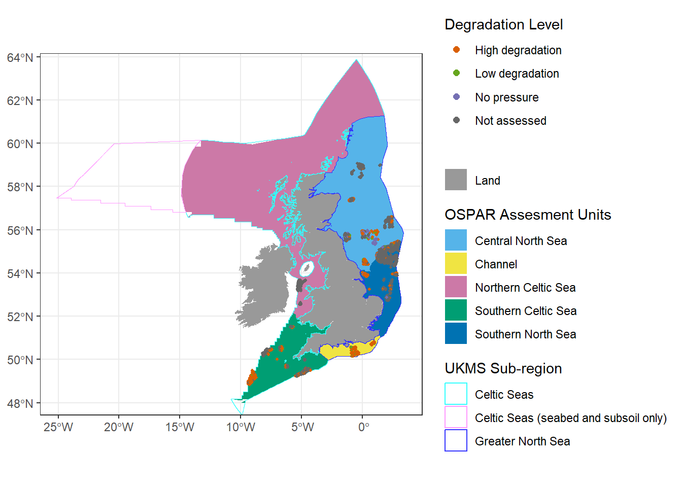
Figure 4. BH1 results at sample level. For each sample point, the degradation level is assessed checking whether the observed proportion of sentinel species is above or below the quality boundary identified from the pressure state curve of the relevant habitat. Assessments are done separately for surface and subsurface abrasion. A sample is considered under low degradation only if the assessed proportion of sentinel species is above the quality boundary for both surface and subsurface abrasion.
Further information
Biological Trait Analysis
The biological dataset included 1103 different taxa belonging to 23 different classes (Table 3). The majority of the taxa recorded in the dataset belonged to the class Polychaeta (41%), followed by Malacostraca (28%), Bivalvia (11%), Gastropoda (9%). The taxa observed within these most common classes tend to be tolerant to trawling pressure (modal BESITO index = 2). All the other classes accounted for a small proportion of the taxa recorded.
Table 3. Composition of the benthic dataset with summary of BESITO values for the classes observed. Note: the table contains NA values for the column ‘class’. These include taxa recorded at phylum level (Nemertea, Platyhelminthes) and taxa belonging to two orders not linked to any class in WoRMS: Priapulomorpha and Sipuncula.
|
Class |
Taxa (n) |
Proportion (%) |
BESITO values by Class |
||
|
Mode |
Mean |
Median |
|||
|
Polychaeta |
454 |
41 |
2 |
2.5 |
2 |
|
Malacostraca |
311 |
28 |
2 |
1.9 |
2 |
|
Bivalvia |
118 |
11 |
2 |
2.7 |
3 |
|
Gastropoda |
98 |
9 |
2 |
2.3 |
2 |
|
Holothuroidea |
21 |
2 |
3 |
3 |
3 |
|
Ophiuroidea |
15 |
1 |
3 |
2.9 |
3 |
|
NA |
13 |
1 |
2 |
2.5 |
2 |
|
Pycnogonida |
12 |
1 |
2 |
2.8 |
2 |
|
Hexacorallia |
11 |
1 |
4 |
4.2 |
4 |
|
Echinoidea |
10 |
1 |
4 |
3.2 |
4 |
|
Asteroidea |
7 |
1 |
3 |
2.4 |
3 |
|
Polyplacophora |
7 |
1 |
2 |
2 |
2 |
|
Clitellata |
6 |
1 |
2 |
2.5 |
2 |
|
Octocorallia |
4 |
0 |
4 |
4 |
4 |
|
Caudofoveata |
3 |
0 |
2 |
2 |
2 |
|
Scaphopoda |
3 |
0 |
2 |
2 |
2 |
|
Solenogastres |
3 |
0 |
2 |
2 |
2 |
|
Enteropneusta |
2 |
0 |
5 |
4 |
4 |
|
Crinoidea |
1 |
0 |
4 |
4 |
4 |
|
Leptocardii |
1 |
0 |
2 |
2 |
2 |
|
Myxini |
1 |
0 |
5 |
5 |
5 |
|
Palaeonemertea |
1 |
0 |
3 |
3 |
3 |
|
Pilidiophora |
1 |
0 |
3 |
3 |
3 |
Sentinel Species Selection
The selection of sentinel species was run for EUNIS Level 3 habitats for each OSPAR benthic assessment unit. The selection was run separately for surface abrasion and subsurface abrasion. The taxa identified as sentinel species on the basis of their sensitivity to trawling pressure are displayed in Table 4.
Table 4. List of sentinel species selected for each combination of EUNIS Level 3 habitat type, OSPAR assessment unit and pressure type. Grey cells indicate cases in which there were insufficient data available to obtain a list of sentinel species (i.e. poor or no data coverage in least impacted areas).
|
Assessment Area |
Habitat Type |
Sentinel Species List (Surface Abrasion) |
Sentinel Species List (Sub-Surface Abrasion) |
|
Central North Sea |
Sublittoral coarse sediment (A5.1) |
Ampelisca spinipes, Ampharete octocirrata, Amphiura filiformis, Galathowenia oculata, Hydroides norvegica, Myriochele, Nemertea, Nototropis vedlomensis, Onchidorididae, Pista cristata, Polycirrus, Sabellaria spinulosa, Scoloplos armiger, Serpulidae, Spirobranchus triqueter, Synarachnactis lloydii, Trichobranchus roseus, Tridonta montagui |
Nototropis vedlomensis, Onchidorididae, Sabellaria spinulosa |
|
Central North Sea |
Sublittoral Sand (A5.2) |
Amphictene auricoma, Amphiura filiformis, Chamelea striatula, Cochlodesma praetenue, Echinocardium flavescens, Edwardsiidae, Galathowenia oculata, Magelona filiformis, Nemertea, Owenia, Scoloplos armiger, Synarachnactis lloydii, Trichobranchus roseus |
Ampelisca tenuicornis, Amphictene auricoma, Amphiura filiformis, Chamelea striatula, Cochlodesma praetenue, Dosinia lupinus, Echinocardium flavescens, Edwardsiidae, Galathowenia oculata, Magelona filiformis, Nemertea, Owenia, Scoloplos armiger, Synarachnactis lloydii, Trichobranchus roseus |
|
Central North Sea |
Sublittoral mud (A5.3) |
Acanthocardia echinata, Ampelisca tenuicornis, Amphictene auricoma, Amphiura filiformis, Cirratulus cirratus, Eunereis longissima, Galathowenia oculata, Glossobalanus marginatus, Leptosynapta inhaerens, Myriochele, Nemertea, Nephtys kersivalensis, Nephtys pente, Oestergrenia digitata, Phyllodoce groenlandica, Pista cristata, Praxillella affinis, Scoloplos armiger, Streblosoma, Synarachnactis lloydii, Terebellidae, Terebellides stroemii, Trichobranchus roseus, Tubulanus polymorphus, Virgularia mirabilis |
Acanthocardia echinata, Ampelisca tenuicornis, Amphictene auricoma, Amphiura filiformis, Cirratulus cirratus, Eunereis longissima, Galathowenia oculata, Glossobalanus marginatus, Leptosynapta inhaerens, Myriochele, Nemertea, Nephtys kersivalensis, Nephtys pente, Oestergrenia digitata, Phyllodoce groenlandica, Pista cristata, Praxillella affinis, Scoloplos armiger, Streblosoma, Synarachnactis lloydii, Terebellidae, Terebellides stroemii, Trichobranchus roseus, Tubulanus polymorphus, Virgularia mirabilis |
|
Central North Sea |
Sublittoral mixed sediments (A5.4) |
Actiniaria, Edwardsiidae, Enteropneusta, Lyonsia norwegica, Musculus subpictus, Nototropis vedlomensis, Onchidorididae, Sabellaria spinulosa |
Actiniaria, Edwardsiidae, Enteropneusta, Lyonsia norwegica, Musculus subpictus, Nototropis vedlomensis, Onchidorididae, Sabellaria spinulosa |
|
Channel |
Sublittoral coarse sediment (A5.1) |
Sabellaria spinulosa |
Ampharete lindstroemi, Cirratulus cirratus, Eulalia mustela, Eumida bahusiensis, Eunereis longissima, Eusyllinae, Glycymeris glycymeris, Leiochone johnstoni, Nemertea, Ophiothrix fragilis, Pherusa plumosa, Polycirrus, Polynoidae, Pseudosyllis brevipennis, Sabellaria spinulosa, Sabellidae, Sphenia binghami, Spirobranchus lamarcki, Spirobranchus triqueter, Spisula elliptica, Tharyx killariensis, Thelepus cincinnatus |
|
Channel |
Sublittoral Sand (A5.2) |
Glycera lapidum, Notomastus |
Glycera lapidum, Notomastus |
|
Channel |
Sublittoral mud (A5.3) |
insufficient data |
insufficient data |
|
Channel |
Sublittoral mixed sediments (A5.4) |
insufficient data |
Caridea, Mimachlamys varia, Sabellaria spinulosa |
|
Northern Celtic Sea |
Sublittoral coarse sediment (A5.1) |
Onchidorididae, Sabellaria spinulosa |
Onchidorididae, Sabellaria spinulosa |
|
Northern Celtic Sea |
Sublittoral Sand (A5.2) |
Actiniaria, Ampelisca spinipes, Ampharete lindstroemi, Amphipholis squamata, Aphelochaeta, Dipolydora caulleryi, Dipolydora coeca, Dipolydora socialis, Eulalia mustela, Eupolymnia nebulosa, Nemertea, Phisidia aurea, Polycirrus, Sabellaria spinulosa, Schistomeringos rudolphi, Spisula elliptica, Terebellides stroemii |
Actiniaria, Ampelisca spinipes, Ampharete lindstroemi, Amphipholis squamata, Aphelochaeta, Dipolydora caulleryi, Dipolydora coeca, Dipolydora socialis, Eulalia mustela, Eupolymnia nebulosa, Nemertea, Nototropis vedlomensis, Phisidia aurea, Polycirrus, Sabellaria spinulosa, Schistomeringos rudolphi, Spisula elliptica, Terebellides stroemii |
|
Northern Celtic Sea |
Sublittoral mud (A5.3) |
insufficient data |
insufficient data |
|
Northern Celtic Sea |
Sublittoral mixed sediments (A5.4) |
Sabellaria spinulosa |
Sabellaria spinulosa |
|
Southern Celtic Sea |
Sublittoral coarse sediment (A5.1) |
insufficient data |
Actiniaria, Decapoda, Edwardsiidae, Hiatella arctica, Lanassa venusta, Metavermilia multicristata, Modiolula phaseolina, Nototropis vedlomensis, Pseudosyllis brevipennis, Sabellaria spinulosa |
|
Southern Celtic Sea |
Sublittoral Sand (A5.2) |
Aonides paucibranchiata, Chone, Galathowenia oculata, Loimia medusa, Nemertea |
Actiniaria, Aspidosiphon (Aspidosiphon) muelleri muelleri, Chone, Galathowenia oculata, Loimia medusa, Lumbrineris aniara, Nemertea, Paraphellia expansa, Pista cristata, Polycirrus, Tubulanus polymorphus |
|
Southern Celtic Sea |
Sublittoral mud (A5.3) |
insufficient data |
Ampelisca spinipes, Ampelisca tenuicornis, Ampharete lindstroemi, Amphiura filiformis, Aspidosiphon (Aspidosiphon) muelleri muelleri, Dasybranchus, Dipolydora coeca, Galathowenia oculata, Kirkegaardia, Magelona alleni, Myriochele, Nemertea, Nephtys kersivalensis, Papillicardium minimum, Paranymphon spinosum, Polycirrus, Pseudonotomastus southerni, Terebellides stroemii, Tharyx killariensis |
|
Southern Celtic Sea |
Sublittoral mixed sediments (A5.4) |
insufficient data |
Actiniaria, Anomiidae, Decapoda, Edwardsiidae, Gnathiidae, Hiatella arctica, Polynoinae, Sabellaria spinulosa, Terebelliformia |
|
Southern North Sea |
Sublittoral coarse sediment (A5.1) |
Amphipholis squamata, Dipolydora caulleryi, Dosinia lupinus, Ensis magnus, Lumbrineris cingulata, Nemertea, Nototropis vedlomensis, Nudibranchia, Pista cristata, Polycirrus, Polynoidae, Spirobranchus lamarcki, Spisula elliptica, Terebellidae, Thracia gracilis |
Amphipholis squamata, Dipolydora caulleryi, Dosinia lupinus, Ensis magnus, Lumbrineris cingulata, Nemertea, Nototropis vedlomensis, Nudibranchia, Polycirrus, Polynoidae, Scoloplos armiger, Spirobranchus lamarcki, Spisula elliptica, Terebellidae, Thracia gracilis |
|
Southern North Sea |
Sublittoral Sand (A5.2) |
Dosinia lupinus, Magelona filiformis, Nemertea, Polycirrus, Polynoidae, Scoloplos armiger, Spatangoida, Terebellidae, Thracia gracilis |
Dosinia lupinus, Magelona filiformis, Nemertea, Polynoidae, Scoloplos armiger, Spatangoida |
|
Southern North Sea |
Sublittoral mud (A5.3) |
insufficient data |
Acrocnida brachiata, Bathyporeia elegans, Bathyporeia guilliamsoniana, Goniada maculata, Magelona johnstoni, Nemertea, Ophelia borealis, Spatangoida, Spiophanes bombyx |
|
Southern North Sea |
Sublittoral mixed sediments (A5.4) |
Actiniaria, Ampelisca diadema, Ampelisca spinipes, Amphipholis squamata, Aphelochaeta, Caulleriella alata, Cirriformia tentaculata, Crepidula fornicata, Dipolydora caulleryi, Eulalia expusilla, Eumida, Eumida bahusiensis, Eunereis longissima, Hiatella arctica, Hydroides norvegica, Hypereteone foliosa, Lumbrineris cingulata, Mya arenaria, Mya truncata, Mytilus edulis, Nemertea, Nephtys kersivalensis, Nuculana minuta, Ophiura albida, Parexogone hebes, Parvicardium pinnulatum, Pherusa plumosa, Phyllodoce groenlandica, Phyllodoce longipes, Polycirrus, Polynoidae, Praxillella affinis, Sabellaria spinulosa, Scoloplos armiger, Serpulidae, Spirobranchus lamarcki, Spisula elliptica, Terebellides, Thelepus cincinnatus, Thyone fusus |
Actiniaria, Ampelisca diadema, Ampelisca spinipes, Amphipholis squamata, Aphelochaeta, Caulleriella alata, Cirriformia tentaculata, Crepidula fornicata, Dipolydora caulleryi, Eulalia expusilla, Eumida, Eumida bahusiensis, Eunereis longissima, Hiatella arctica, Hydroides norvegica, Hypereteone foliosa, Lumbrineris cingulata, Mya arenaria, Mya truncata, Mytilus edulis, Nemertea, Nephtys kersivalensis, Nuculana minuta, Ophiura albida, Parexogone hebes, Parvicardium pinnulatum, Pherusa plumosa, Phyllodoce groenlandica, Phyllodoce longipes, Polycirrus, Polynoidae, Praxillella affinis, Sabellaria spinulosa, Scoloplos armiger, Serpulidae, Spirobranchus lamarcki, Spisula elliptica, Terebellides, Thelepus cincinnatus, Thyone fusus |
Changes in sentinel species proportion with pressure
Due to low number of samples, high number of ties (two or more observations that have the same value) and uneven distribution of the data within the datasets, the Kendall’s Tau correlation was used to assess the relationship between sentinel species proportion of sample biomass and the pressure gradients.
DETAILED RESULTS AT THE OSPAR ASSESSMENT UNIT WITHIN UK WATERS SCALE
Central North Sea
In this assessment unit, most of the pressure/state relationships obtained were either not significant or unreliable (Table 5). Sublittoral sand was the only habitat type for which reliable quality boundaries could be obtained. This habitat showed linear response to surface abrasion and a tolerant response to subsurface.
Table 5. Overall summary of the BH1 analysis in the Central North Sea. For each combination EUNIS Level 3 habitat and pressure type, we reported the habitat sensitivity (mean ± standard deviation) with the resultant habitat response type. Precautionary, standard, tolerant boundaries and tipping point values obtained from each pressure-state curve are also provided, with numbers reflecting the habitat quality loss level and values between parenthesis defining the pressure level at each boundary. Blue Cells indicate the quality boundary selected based on the habitat sensitivity. Grey cells indicate cases in which quality boundaries could not be identified because there were insufficient data to calculate pressure/state relationships or because the relationships identified were either not significant, not reliable or returned null values. N/A = not assessed.
|
EUNIS Habitat |
Trawling Abrasion Type |
Habitat Sensitivity |
Standard Deviation |
Precuationary Boundary |
Standard Boundary |
Tolerant Boundary |
Tipping Point |
Habitat Response Type |
Pressure-State Curve Review |
|
Sublittoral coarse sediment (A5.1) |
Surface |
N/A |
N/A |
N/A |
N/A |
N/A |
N/A |
Tolerant |
unreliable model |
|
Sublittoral sand (A5.2) |
Surface |
3.231 |
0.54 |
0.7 (0.5) |
0.55 (0.8) |
0.4 (1.2) |
0.1 (2.96) |
linear |
reliable pressure-state model |
|
Sublittoral mud (A5.3) |
Surface |
N/A |
N/A |
N/A |
N/A |
N/A |
N/A |
linear |
unreliable model |
|
Sublittoral mixed sediments (A5.4) |
Surface |
N/A |
N/A |
N/A |
N/A |
N/A |
N/A |
linear |
non-significant correlation |
|
Sublittoral coarse sediment (A5.1) |
Subsurface |
N/A |
N/A |
N/A |
N/A |
N/A |
N/A |
sensitive |
non-significant correlation |
|
Sublittoral sand (A5.2) |
Subsurface |
2.138 |
0.74 |
0.68 (0.2) |
0.52 (0.3) |
0.36 (0.5) |
0.04 (1.63) |
Tolerant |
reliable pressure-state model |
|
Sublittoral mud (A5.3) |
Subsurface |
N/A |
N/A |
N/A |
N/A |
N/A |
N/A |
linear |
unreliable model |
|
Sublittoral mixed sediments (A5.4) |
Subsurface |
N/A |
N/A |
N/A |
N/A |
N/A |
N/A |
Tolerant |
non-significant correlation |
687 samples were available in this assessment unit, 26% of which represented high degradation, 3% low degradation and 55% were not assessed, 15% of samples were found to have no pressure (Figure 5).
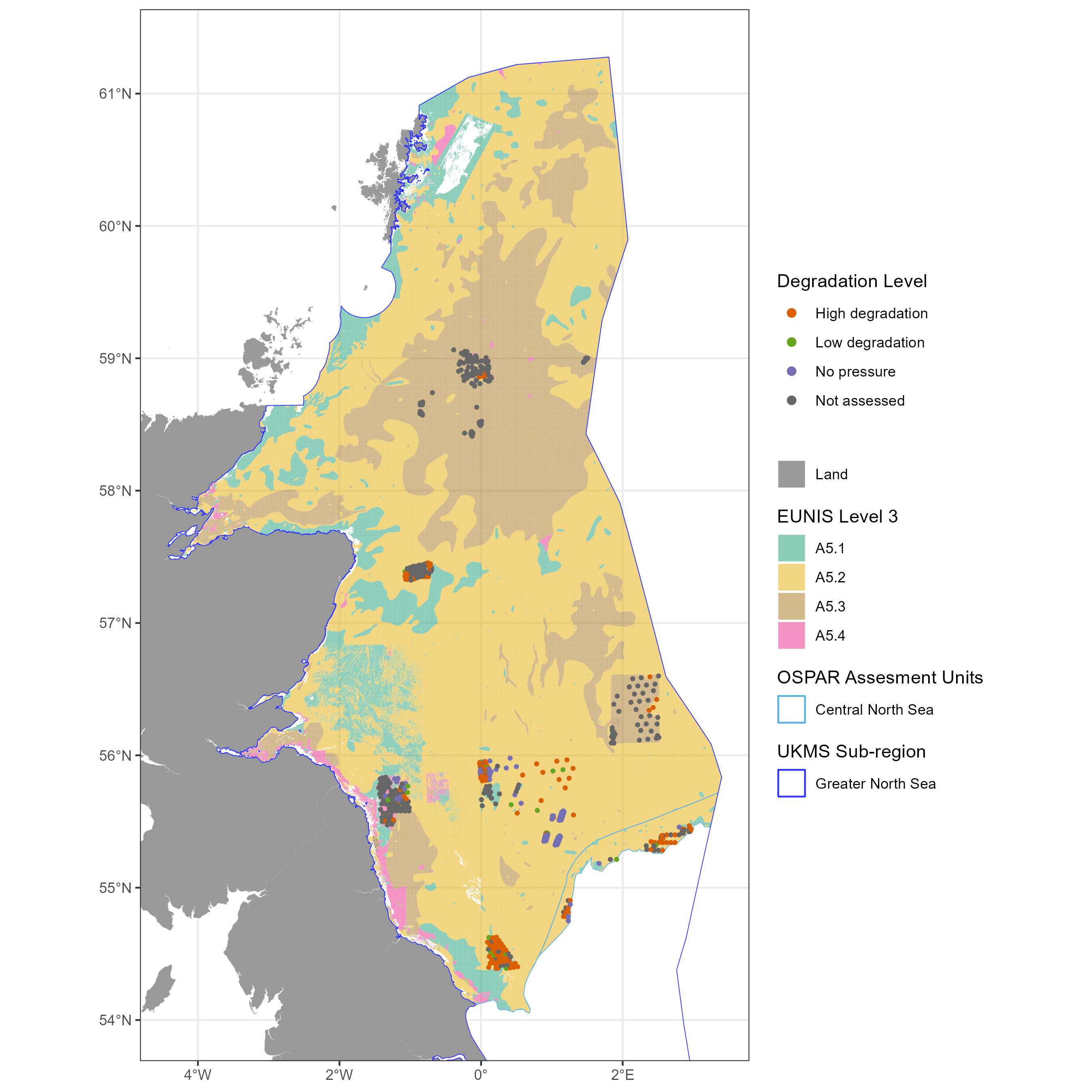
Figure 5. Distribution of benthic sample points, and their estimated degradation level, throughout the Central North Sea.
Southern North Sea
In this assessment unit, reliable quality boundaries could be defined for sublittoral mixed sediments and for sublittoral mud (subsurface only) (Table 6). Sublittoral mixed sediments showed a sensitive response to surface and subsurface pressure, whilst sublittoral mud showed a linear response to subsurface abrasion from bottom-contacting fisheries.
Table 6. Overall summary of the BH1 analysis in the Southern North Sea. For each combination EUNIS Level 3 habitat and pressure type, we reported the habitat sensitivity (mean ± standard deviation) with the resultant habitat response type. Precautionary, standard, tolerant boundaries and tipping point values obtained from each pressure-state curve are also provided, with numbers reflecting the habitat quality loss level and values between parenthesis defining the pressure level at each boundary. Blue Cells indicate the quality boundary selected based on the habitat sensitivity. Grey cells indicate cases in which quality boundaries could not be identified because there were insufficient data to calculate pressure/state relationships or because the relationships identified were either not significant, not reliable or returned null values. N/A = not assessed.
|
EUNIS Habitat |
Trawling Abrasion Type |
Habitat Sensitivity |
Standard Deviation |
Precuationary Boundary |
Standard Boundary |
Tolerant Boundary |
Tipping Point |
Habitat Response Type |
Pressure-State Curve Review |
|
Sublittoral coarse sediment (A5.1) |
Surface |
N/A |
N/A |
N/A |
N/A |
N/A |
N/A |
linear |
unreliable model |
|
Sublittoral sand (A5.2) |
Surface |
N/A |
N/A |
N/A |
N/A |
N/A |
N/A |
Tolerant |
non-significant correlation |
|
Sublittoral mud (A5.3) |
Surface |
N/A |
N/A |
N/A |
N/A |
N/A |
N/A |
N/A |
insufficient data |
|
Sublittoral mixed sediments (A5.4) |
Surface |
3.686 |
0.49 |
0.72 (0.5) |
0.58 (0.8) |
0.44 (1.2) |
0.16 (2.97) |
sensitive |
reliable pressure-state model |
|
Sublittoral coarse sediment (A5.1) |
Subsurface |
N/A |
N/A |
N/A |
N/A |
N/A |
N/A |
Tolerant |
non-significant correlation |
|
Sublittoral sand (A5.2) |
Subsurface |
N/A |
N/A |
N/A |
N/A |
N/A |
N/A |
Tolerant |
non-significant correlation |
|
Sublittoral mud (A5.3) |
Subsurface |
3.136 |
0.72 |
0.7 (0.4) |
0.54 (0.8) |
0.39 (1.2) |
0.09 (2.93) |
linear |
reliable pressure-state model |
|
Sublittoral mixed sediments (A5.4) |
Subsurface |
3.663 |
0.52 |
0.7 (0.2) |
0.55 (0.4) |
0.4 (0.6) |
0.1 (1.87) |
sensitive |
reliable pressure-state model |
A total of 725 grab samples were available in this assessment unit, mostly concentrated in the northwest of the assessment unit, which corresponds with the location of Dogger Bank Special Area of Conservation (Figure 6). Among available samples, 10% represented high degradation, <1% low degradation, 86% were not assessed, and 4% had no pressure. Where samples were assessed for sublittoral mud and sublittoral mixed sediments, the majority of samples were classed as highly degraded, 100% and 63%, respectively.
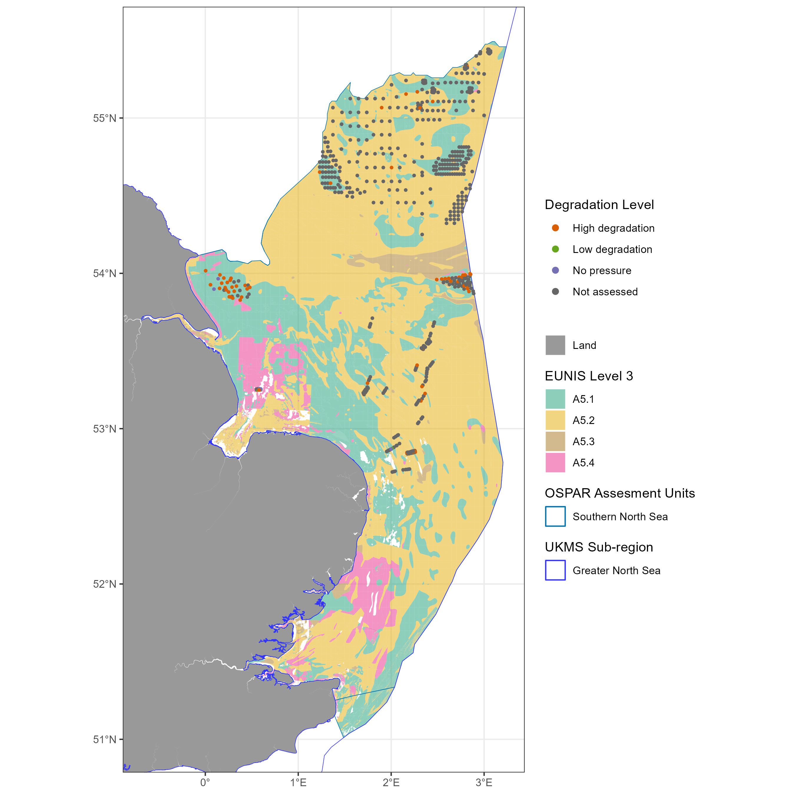
Figure 6. Distribution of benthic sample points, and their estimated degradation level, throughout the Southern North Sea.
Channel
In this assessment unit, reliable quality boundaries were obtained for sublittoral coarse sediment and sublittoral sand (surface and subsurface) and for sublittoral mixed sediments (subsurface only) (Table 7). All habitats assessed showed a sensitive response to pressure. No assessments could be made for sublittoral mud due to lack of data.
Table 7. Overall summary of the BH1 analysis in the Channel. For each combination EUNIS Level 3 habitat and pressure type, we reported the habitat sensitivity (mean ± standard deviation) with the resultant habitat response type. Precautionary, standard, tolerant boundaries and tipping point values obtained from each pressure-state curve are also provided, with numbers reflecting the habitat quality loss level and values between parenthesis defining the pressure level at each boundary. Blue Cells indicate the quality boundary selected based on the habitat sensitivity. Grey cells indicate cases in which quality boundaries could not be identified because there were insufficient data to calculate pressure/state relationships or because the relationships identified were either not significant, not reliable or returned null values. N/A = not assessed.
|
EUNIS Habitat |
Trawling Abrasion Type |
Habitat Sensitivity |
Standard Deviation |
Precuationary Boundary |
Standard Boundary |
Tolerant Boundary |
Tipping Point |
Habitat Response Type |
Pressure-State Curve Review |
|
Sublittoral coarse sediment (A5.1) |
Surface |
3.533 |
0.57 |
0.71 (0.6) |
0.56 (1) |
0.42 (1.5) |
0.13 (3.55) |
sensitive |
reliable pressure-state model |
|
Sublittoral sand (A5.2) |
Surface |
3.82 |
0.41 |
0.69 (0.7) |
0.54 (1.1) |
0.39 (1.5) |
0.08 (3.27) |
sensitive |
reliable pressure-state model |
|
Sublittoral mud (A5.3) |
Surface |
N/A |
N/A |
N/A |
N/A |
N/A |
N/A |
N/A |
insufficient data |
|
Sublittoral mixed sediments (A5.4) |
Surface |
N/A |
N/A |
N/A |
N/A |
N/A |
N/A |
N/A |
insufficient data |
|
Sublittoral coarse sediment (A5.1) |
Subsurface |
3.874 |
0.33 |
0.68 (0.3) |
0.52 (0.4) |
0.35 (0.6) |
0.03 (1.67) |
sensitive |
reliable pressure-state model |
|
Sublittoral sand (A5.2) |
Subsurface |
3.715 |
0.46 |
0.68 (0.4) |
0.52 (0.6) |
0.36 (0.9) |
0.04 (2.1) |
sensitive |
reliable pressure-state model |
|
Sublittoral mud (A5.3) |
Subsurface |
N/A |
N/A |
N/A |
N/A |
N/A |
N/A |
N/A |
insufficient data |
|
Sublittoral mixed sediments (A5.4) |
Subsurface |
4.279 |
0.74 |
0.67 (0) |
0.5 (0.1) |
0.34 (0.1) |
0.01 (0.67) |
sensitive |
reliable pressure-state model |
In the Channel there were 150 samples available of which 95% were considered highly degraded and the remaining 5% represented low degradation (Figure 7). This assessment unit represented the only assessment unit were 100% of samples could be assessed for degradation. The majority of samples in all three habitats assessed were classed as highly degraded: sublittoral coarse sediment (98%), sublittoral sand (95%) and sublittoral mixed sediments (90%).
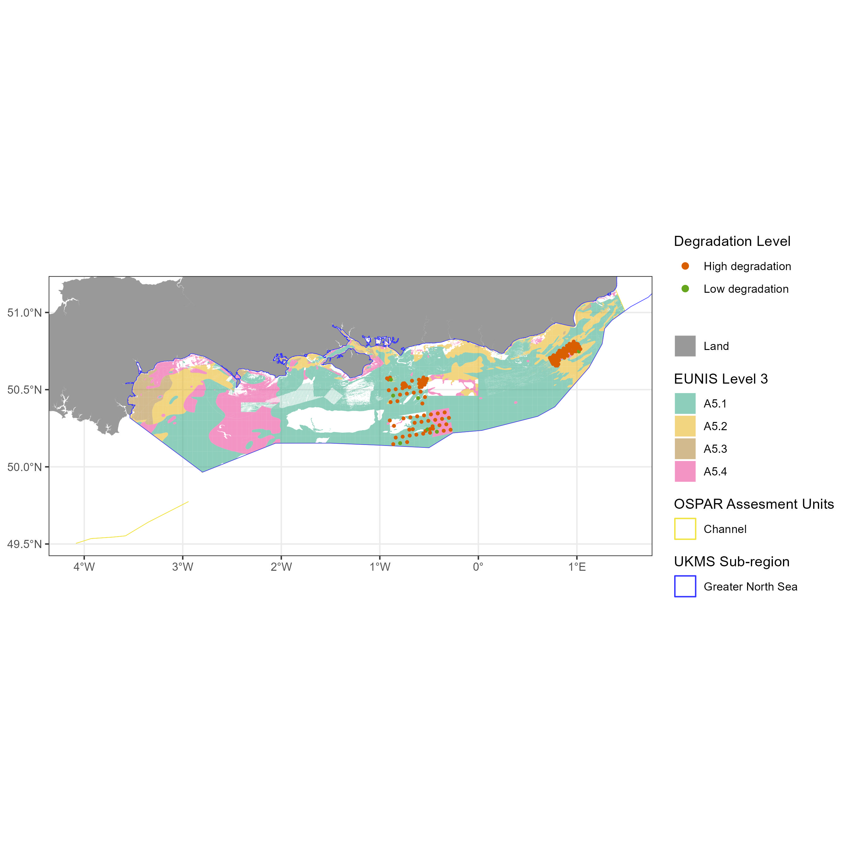
Figure 7. Distribution of benthic sample points, and their estimated degradation level, throughout the Channel.
Northern Celtic Sea
In this assessment unit, data were insufficient to extract sentinel species lists in most of the cases and, when possible, the resulting pressure-state curves were not significant (Table 8).
Table 8. Overall summary of the BH1 analysis in the Northern Celtic Sea. For each combination EUNIS Level 3 habitat and pressure type, we reported the habitat sensitivity (mean ± standard deviation) with the resultant habitat response type. Precautionary, standard, tolerant boundaries and tipping point values obtained from each pressure-state curve are also provided, with numbers reflecting the habitat quality loss level and values between parenthesis defining the pressure level at each boundary. Blue Cells indicate the quality boundary selected based on the habitat sensitivity. Grey cells indicate cases in which quality boundaries could not be identified because there were insufficient data to calculate pressure/state relationships or because the relationships identified were either not significant, not reliable or returned null values. N/A = not assessed.
|
EUNIS Habitat |
Trawling Abrasion Type |
Habitat Sensitivity |
Standard Deviation |
Precuationary Boundary |
Standard Boundary |
Tolerant Boundary |
Tipping Point |
Habitat Response Type |
Pressure-State Curve Review |
|
Sublittoral coarse sediment (A5.1) |
Surface |
N/A |
N/A |
N/A |
N/A |
N/A |
N/A |
N/A |
insufficient data |
|
Sublittoral sand (A5.2) |
Surface |
N/A |
N/A |
N/A |
N/A |
N/A |
N/A |
N/A |
non-significant correlation |
|
Sublittoral mud (A5.3) |
Surface |
N/A |
N/A |
N/A |
N/A |
N/A |
N/A |
N/A |
insufficient data |
|
Sublittoral mixed sediments (A5.4) |
Surface |
N/A |
N/A |
N/A |
N/A |
N/A |
N/A |
N/A |
non-significant correlation |
|
Sublittoral coarse sediment (A5.1) |
Subsurface |
N/A |
N/A |
N/A |
N/A |
N/A |
N/A |
N/A |
insufficient data |
|
Sublittoral sand (A5.2) |
Subsurface |
N/A |
N/A |
N/A |
N/A |
N/A |
N/A |
N/A |
non-significant correlation |
|
Sublittoral mud (A5.3) |
Subsurface |
N/A |
N/A |
N/A |
N/A |
N/A |
N/A |
N/A |
insufficient data |
|
Sublittoral mixed sediments (A5.4) |
Subsurface |
N/A |
N/A |
N/A |
N/A |
N/A |
N/A |
N/A |
non-significant correlation |
Available sample data covered a small proportion of this assessment unit, with only 159 samples concentrated in the waters around Wales (Figure 8). A quality boundary could not be determined for any of the 159 samples in the assessment unit and therefore no samples were able to be assessed.
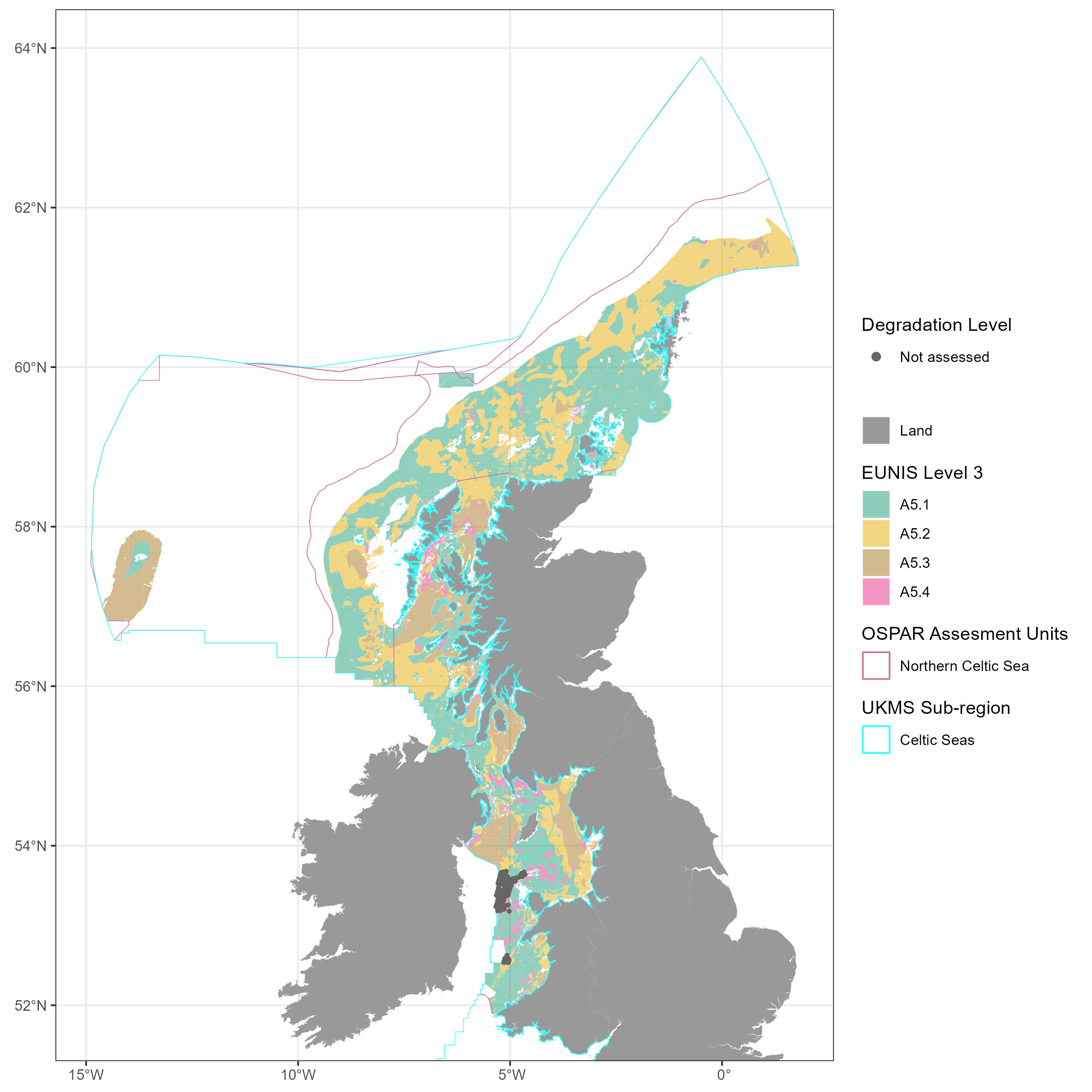
Figure 8. Distribution of benthic sample points, and their estimated degradation level, throughout the Northern Celtic Sea.
Southern Celtic Sea
In this assessment unit, data were insufficient to extract sentinel species lists in many cases and, when possible, the resulting pressure-state curves were sometimes not significant (Table 9). Reliable quality boundaries could be determined for sublittoral sand, which showed a linear response to surface abrasion and sensitive response to subsurface, and for sublittoral mixed sediments (subsurface only), which showed a sensitive response to subsurface abrasion.
Table 9. Overall summary of the BH1 analysis in the Southern Celtic Sea. For each combination EUNIS Level 3 habitat and pressure type, we reported the habitat sensitivity (mean ± standard deviation) with the resultant habitat response type. Precautionary, standard, tolerant boundaries and tipping point values obtained from each pressure-state curve are also provided, with numbers reflecting the habitat quality loss level and values between parenthesis defining the pressure level at each boundary. Blue Cells indicate the quality boundary selected based on the habitat sensitivity. Grey cells indicate cases in which quality boundaries could not be identified because there were insufficient data to calculate pressure/state relationships or because the relationships identified were either not significant, not reliable or returned null values. N/A = not assessed.
|
EUNIS Habitat |
Trawling Abrasion Type |
Habitat Sensitivity |
Standard Deviation |
Precautionary Boundary |
Standard Boundary |
Tolerant Boundary |
Tipping Point |
Habitat Response Type |
Pressure-State Curve Review |
|
Sublittoral coarse sediment (A5.1) |
Surface |
N/A |
N/A |
N/A |
N/A |
N/A |
N/A |
N/A |
insufficient data |
|
Sublittoral sand (A5.2) |
Surface |
2.131 |
1.17 |
0.92 (0.8) |
0.88 (1.2) |
0.85 (1.5) |
0.77 (2.54) |
linear |
reliable pressure-state model |
|
Sublittoral mud (A5.3) |
Surface |
N/A |
N/A |
N/A |
N/A |
N/A |
N/A |
N/A |
insufficient data |
|
Sublittoral mixed sediments (A5.4) |
Surface |
N/A |
N/A |
N/A |
N/A |
N/A |
N/A |
N/A |
insufficient data |
|
Sublittoral coarse sediment (A5.1) |
Subsurface |
N/A |
N/A |
N/A |
N/A |
N/A |
N/A |
N/A |
non-significant correlation |
|
Sublittoral sand (A5.2) |
Subsurface |
3.777 |
0.45 |
0.7 (0.1) |
0.56 (0.1) |
0.41 (0.2) |
0.11 (0.96) |
sensitive |
reliable pressure-state model |
|
Sublittoral mud (A5.3) |
Subsurface |
N/A |
N/A |
N/A |
N/A |
N/A |
N/A |
N/A |
non-significant correlation |
|
Sublittoral mixed sediments (A5.4) |
Subsurface |
2.56 |
1.77 |
0.68 (0.7) |
0.52 (0.8) |
0.37 (0.9) |
0.05 (1.59) |
sensitive |
reliable pressure-state model |
370 samples were available, 59% of which were highly degraded, 1% of were classed as low degradation, and 39% not assessed (Figure 9). Where samples from habitats were able to be assessed (sublittoral sand and sublittoral mixed sediments) the majority were classed as high degradation (98% and 97% respectively), with 2% and 3% of samples classed as low degradation.
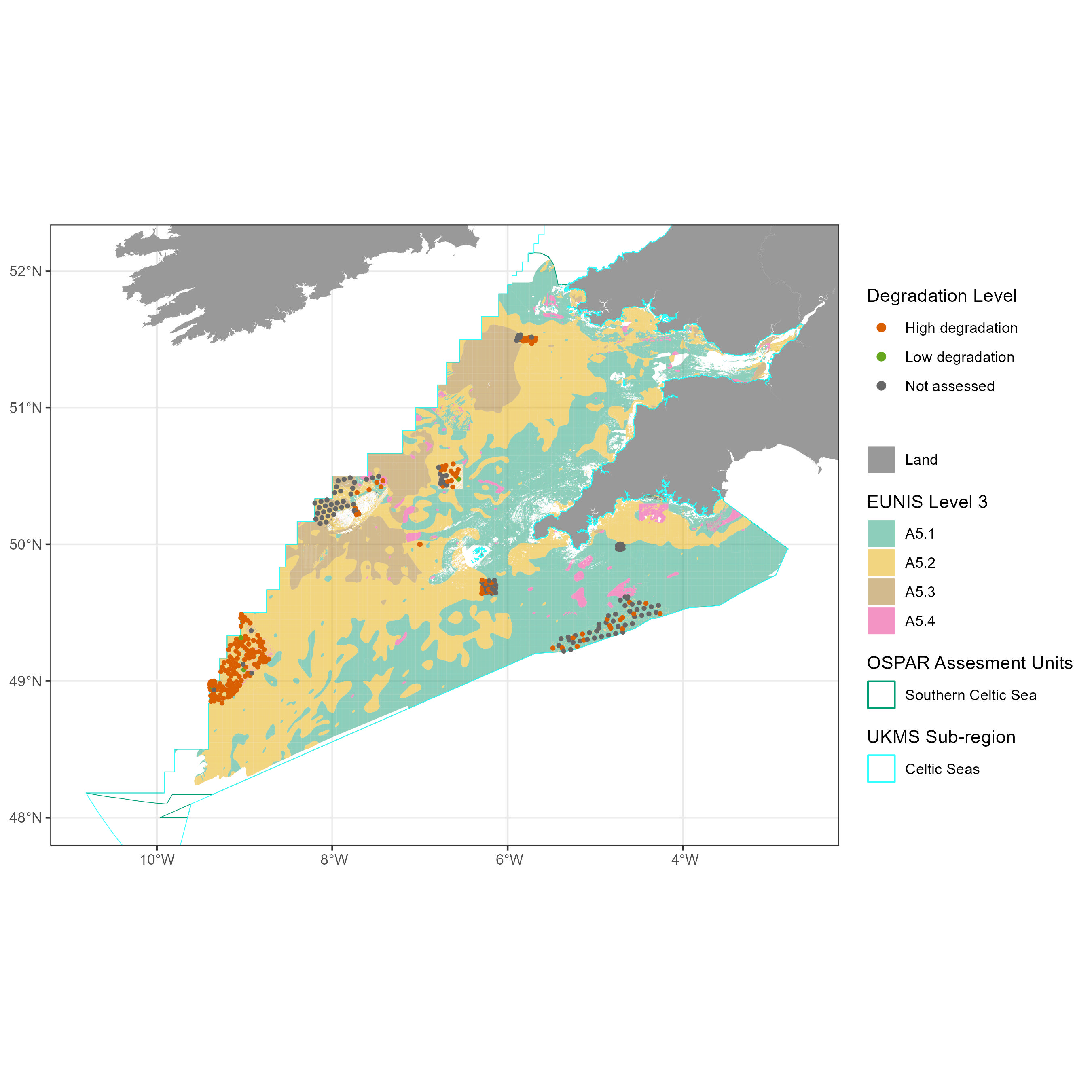
Figure 9. Distribution of benthic sample points, and their estimated degradation level, throughout the Southern Celtic Sea.
Conclusions
This pilot assessment applied the OSPAR indicator ‘Sentinels of the Seabed’ to the Celtic Seas and Greater North Sea sub-regions. Where habitat condition could be assessed, the majority of samples indicated high levels of degradation in the two sub-regions. Due to limitations from the monitoring programme, habitat condition could not be assessed for a large proportion of available samples, 51% in the Celtic Seas sub-region and 64% in the Greater North Sea sub-region. Monitoring data in the UK are very clustered, particularly around MPAs, with little coverage of the pressure gradient. This impaired the possibility to obtain significant and reliable pressure-state relationships which require data collection across different levels of exposure to pressure. It should be considered that this pilot assessment was based on data collected from a single grab type (0.1 m2 Hamon grabs) and does not consider potentially useful data collected with different sampling gears. Future iterations should evaluate the possibility to consider additional sampling gears in the analyses to provide more comprehensive assessments.
The indicator has strong potential for the assessment of change in habitat condition and function and is useful to detect quality boundaries and tipping points that could be used for the calibration of model-based indicators that rely on a risk assessment approach to cover large areas of sea without direct monitoring data, in particular BH3a ‘Extent of Physical Disturbance’.
Further information
Although thresholds for Good Environmental Status (GES) have not yet been agreed for this pilot indicator, the current assessment provides some initial indication of thresholds ranges, as well as areas where additional monitoring should take place for the next round of assessments. Further method development would be needed to undertake a full GES assessment using this indicator in UK waters.
Knowledge gaps
The following caveats are associated with the pressure data used for this assessment:
-
Pressure information is available at 0.05° x 0.05° c-square resolution and homogeneous trawling intensity and distribution is assumed across each c-square.
-
Limited confidence in the pressure information in coastal areas, where small vessels (< 12m length) are most likely to operate and for which VMS data are currently unavailable.
-
There is a need to better identify impacts from other pressures and natural environmental drivers how these might influence results.
Additionally, there is a need to adapt existing monitoring programmes to collect data across different pressure levels of human activities.
Further information
Various shortcomings of the BH1 method and data sources will need to be addressed in future assessments in order to assess GES and to inform management measures:
Distribution of monitoring data
The spatial distribution of UK data was not ideal to obtain good pressure/state relationships, survey data are: i) very clustered to Marine Protected Areas ii) not ubiquitously distributed across the pressure gradient, and iii) affected by the presence of outliers (which might be indicative of other pressures occurring and/or caused by natural spatial variability in the benthic community). These factors affect the outcome of inference methods used to define pressure state relationships, such as the Generalised Additive Models (GAMs). GAMs are very sensitive to outliers in cases of low replication. Increasing the available monitoring data, including spatial distribution, to input into the indicator might address this limitation. To potentially increase the spatial coverage of benthic data in future assessments with the BH1 indicator, exploratory analyses could be conducted on the use of abundance data, which is more commonly available than biomass data; and data collected with different sampling gears.
Using pressure level as a proxy for condition
This pilot assessment did not attempt to evaluate habitat condition beyond areas covered by biological sample data. Caution should be exercised if plotting results for habitat areas that extend beyond the area covered by monitoring data. A confidence assessment method that includes consideration of the spatial representation of the monitoring data should be developed.
Sensitivity assessment based on the BESITO index and recalibration
The selection of sentinel species is based on their sensitivity to pressure. For demersal trawling the BESITO index was used, which is optimised for benthic epifaunal species rather than infaunal species. The index focusses on eight biological traits that are scored and combined into a unique index of sensitivity.
The formula to calculate the BESITO index assign different weights (1-3) to individual traits, these weightings were defined looking at the strength in traits’ relationship to trawling pressure Gonzalez and others (2018). A large proportion of UK monitoring data was collected using grabs, which are particularly effective at collecting infauna, and less successful at collecting epifauna. Given that UK data are largely collected using grabs, it would be useful to recalibrate the BESITO to ensure that appropriate weightings are assigned for infauna data.
Comparison of BESITO with alternative sensitivity scoring systems
This pilot assessment applied the method developed for the OSPAR QSR 2023 using the BESITO index to assess species sensitivity to trawling. The BESITO index uses a particular trait scoring system to calculate sensitivity. However, there are other trait databases in the UK that use different categories from those considered in BESITO, for example BIOTIC, the Cefas database and the Marine Evidence based Sensitivity Assessment (MarESA) (the latter being used for BH3 indicator as well). It would be useful to evaluate how sensitivity categories used by the different systems are related and investigate if any amendments in the BH1 scoring system are required to increase applicability to UK data.
Lack of ‘true’ reference areas.
In UK waters, areas not impacted by trawling pressure are extremely rare. Therefore, within some habitats, there were an insufficient number of samples within areas of zero pressure to enable sentinel species to be identified from true reference conditions. Thus, in some cases, sentinel species had to be selected from areas considered to be subject to very low pressure. However, even if pressure intensity was very low in these areas, highly sensitive species may have already been negatively impacted and too rare to be included in the sentinel species list.
Additionally, knowledge gaps associated with the available fishing pressure data reduced confidence in the identification of true reference areas. As fishing pressure data did not represent all vessels operational in UK waters (no data for vessel < 12 m in length and no data for vessels < 15 m in length prior to 1st of January 2012), there is a possibility reference conditions were identified in areas where smaller vessels were in operation. However, such instances are more likely in inshore areas, where vessels less than 12 m in length are more prevalent. Furthermore, the assumption that fishing pressure was distributed homogenously throughout each c-square may have overestimated the extent and underestimated the intensity of fishing pressure in some locations. Consequently, future assessments would benefit from: the availability of data for vessels less than 12 m in length, to increase the confidence that areas with zero pressure were truly unaffected by mobile bottom-contact fisheries; and increased resolution of fishing pressure data to improve spatial alignment between benthic samples and SAR values.
Moving beyond the selection of species lists
The BH1 indicator focuses on the identification of habitat-specific species lists (the sentinel species) whose changes in proportion within the benthic community are assessed across a pressure gradient. The focus on individual species has some criticalities associated:
-
Benthic community composition is highly variable for some sediment habitat types, and there may be spatial variability in the composition of the characterising and sensitive species driven by the influence of substrate, natural environmental drivers and geographical factors, such as an area of rock with a thin layer of sediment. The variability in species composition and the effect of spatial and environmental drivers of change need to be accounted for in future analyses.
-
Climatic drivers also need to be considered in the future, such as variations of sea temperature, particularly for those cold water species at the southern limit of their distribution. Climatic drivers might also affect the presence of specific taxa in the future; therefore, caution should be exercised when comparing sentinel species abundance between time intervals.
-
Limitations derived by low data availability could be partially addressed by considering functional groups or sensitivity categories or rather than individual species for assessments. For instance, different species compositions are likely to be observed within benthic communities from different areas, but a common attribute between samples should be that the most sensitive taxa are more abundant in the least impacted areas regardless of the identity of these taxa. It would be beneficial to evaluate the performance of the indicator without focusing on species lists.
References
Clare, D. S., Bolam, S. G., McIlwaine, P. S. O., Garcia, C., Murray, J. M., Eggleton, J. D. 2022. Biological traits of marine benthic invertebrates in Northwest Europe. Scientific Data 9: 339.
De Cáceres, M., Legendre, P., 2009. Associations between species and groups of sites: indices and statistical inference. Ecology, 90, 3566-3574.
De Cáceres, M., Legendre, P., and Moretti, M., 2010. Improving Indicator species analysis by combining groups of sites. Oikos 119: 1674-1684.
Dufrene, M., and Legendre, P., 1997. Species Assemblages and Indicator Species: The Need for a Flexible Asymmetrical Approach. Ecological Monographs, 67(3), 345-366.
Elliott, S.A., Guérin, L., Pesch, R., Schmitt, P., Meakins, B., Vina-Herbon, C., González-Irusta, J.M., de la Torriente, A. and Serrano, A. 2018. Integrating benthic habitat indicators: working towards an ecosystem approach. Marine Policy, 90, 88-94.
González-Irusta, J. M., De la Torriente, A., Punzón, A., Blanco, M., and Serrano, A. 2018. Determining and mapping species sensitivity to trawling impacts: the BEnthos Sensitivity Index to Trawling Operations (BESITO). ICES Journal of Marine Science 75, 1710-1721
ICES, 2021. OSPAR request on the production of spatial data layers of fishing intensity / pressure. ICES Technical service.
Matear, L, Pinder, J. and Lillis, H. 2019. Method for updating the UK full-coverage EUNIS level 3 seabed habitat map integrating fine- and broad-scale maps. https://hub.jncc.gov.uk/assets/538e8eaa-83cc-40cf-bc5a-ef599a716b79
Matear, L., Vina-Herbon, C., Woodcock, K.A., Duncombe-Smith, S.W., Smith, A.P., Schmitt, P., Kreutle, A., Marra, S., Curtis, E.J., and Baigent, H.N. 2023. Extent of Physical Disturbance to Benthic Habitats: Fisheries. In: OSPAR, 2023: The 2023 Quality Status Report for the Northeast Atlantic. OSPAR Commission, London. Available at: https://oap.ospar.org/en/ospar-assessments/quality-status-reports/qsr-2023/indicator-assessments/phys-dist-habs-fisheries/
Plaza-Morlote, M., García-Alegre, A., González-Irusta, J. M., Torriente, A., Fernández-Arcaya, U., Punzón, A. and Serrano, A. 2023. Sentinels of the Seabed. In: OSPAR, 2023: The 2023 Quality Status Report for the North-East Atlantic. OSPAR Commission, London. Available at: https://oap.ospar.org/en/ospar-assessments/quality-status-reports/qsr-2023/indicator-assessments/sentinels-seabed/
Warton, David I., Stephen T. Wright, and Yi Wang. ‘Distance‐based multivariate analyses confound location and dispersion effects.’ Methods in Ecology and Evolution 3, no. 1 (2012): 89-101.
Worsfold, T.M., Hall, D.J. & O'Reilly, M. (Ed.). 2023. Development of standard recording policies for laboratory analysis of north-east Atlantic macrobenthos samples, including a draft Taxonomic Discrimination Protocol (TDP) down to Family level. Report to the NMBAQC Scheme participants. 48pp, August 2023.
Authors
Stefano Marra1, Kirsty Woodcock1, Adam Smith1, Stephen Duncombe-Smith1, Marco Fusi1, Nadia Reeve1, Megan Parry1, Lorna McKellar2, Jenny Booth1, Liam Matear1, Laura Pettit1 and Cristina Vina-Herbon1
1Joint Nature Conservation Committee
2Bangor University
Supported by: The Benthic Sub-Group of the Healthy and Biologically Diverse Seas Evidence Group.
Assessment metadata
| Assessment Type | UK Marine Strategy |
|---|---|
Benthic Habitats | |
| Point of contact email | marinestrategy@defra.gov.uk |
| Metadata date | Monday, January 1, 0001 |
| Title | Pilot Assessment of Sentinels of the Seabed in the Celtic Seas and Greater North Sea |
| Resource abstract | |
| Linkage | Plaza-Morlote, M., García-Alegre, A., González-Irusta, J. M., Torriente, A., Fernández-Arcaya, U., Punzón, A. and Serrano, A. 2023. Sentinels of the Seabed. In: OSPAR, 2023: The 2023 Quality Status Report for the North-East Atlantic. OSPAR Commission, London. Available at: https://oap.ospar.org/en/ospar-assessments/quality-status-reports/qsr-2023/indicator-assessments/sentinels-seabed/
OSPAR Commission (2023). OSPAR Coordinated Environmental Monitoring Programme (CEMP) Guidelines. Common indicator: Common Indicator Sentinels of the Seabed (SoS). Available at: https://www.ospar.org/documents?v=51126 |
| Conditions applying to access and use | Please contact marinestrategy@defra.gov.uk |
| Assessment Lineage | |
| Dataset metadata | Please contact marinestrategy@defra.gov.uk |
| Dataset DOI | Marine Recorder (Public) snapshot version 52 ‘2021-08-09’
Data for OSPAR request on the production of spatial data layers of fishing intensity/pressure |
The Metadata are “data about the content, quality, condition, and other characteristics of data” (FGDC Content Standard for Digital Geospatial Metadata Workbook, Ver 2.0, May 1, 2000).
Metadata definitions
Assessment Lineage - description of data sets and method used to obtain the results of the assessment
Dataset – The datasets included in the assessment should be accessible, and reflect the exact copies or versions of the data used in the assessment. This means that if extracts from existing data were modified, filtered, or otherwise altered, then the modified data should be separately accessible, and described by metadata (acknowledging the originators of the raw data).
Dataset metadata – information on the data sources and characteristics of data sets used in the assessment (MEDIN and INSPIRE compliance).
Digital Object Identifier (DOI) – a persistent identifier to provide a link to a dataset (or other resource) on digital networks. Please note that persistent identifiers can be created/minted, even if a dataset is not directly available online.
Indicator assessment metadata – data and information about the content, quality, condition, and other characteristics of an indicator assessment.
MEDIN discovery metadata - a list of standardized information that accompanies a marine dataset and allows other people to find out what the dataset contains, where it was collected and how they can get hold of it.